4.1: Map Representations

In order to plan a path, we somehow need to represent the environment in the computer. We differentiate between two complementary approaches: discrete and continuous approximations. In a discrete approximation, a map is sub-divided into chunks of equal (e.g., a grid or hexagonal map) or differing sizes (e.g., rooms in a building). The latter maps are also known as topological maps. Discrete maps lend themselves well to a graph representation. Here, every chunk of the map corresponds to a vertex (also known as “node”), which are connected by edges, if a robot can navigate from one vertex to the other. For example a road-map is a topological map, with intersections as vertices and roads as edges, labeled with their length (Figure 4.2.1). Computationally, a graph might be stored as an adjacency or incidence list/matrix. A continuous approximation requires the definition of inner (obstacles) and outer boundaries, typically in the form of a polygon, whereas paths can be encoded as sequences of points defined by real numbers. Despite the memory advantages of a continuous representation, discrete maps are the dominant representation in robotics.

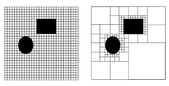
For mapping obstacles, the most common map is the occupancy grid map. In a grid map, the environment is discretized into squares of arbitrary resolution, e.g. 1cm x 1cm, on which obstacles are marked. In a probabilistic occupancy grid, grid cells can also be marked with the probability that they contain an obstacle. This is particularly important when the position of the robot that senses an obstacle is uncertain. Disadvantages of grid maps are their large memory requirements as well as computational time to traverse data structures with large numbers of vertices. A solution to this is storing the grid map as k-d tree. A k-d tree recursively breaks the environment into k pieces. For k = 4, an area is broken into four pieces. Each of these pieces is again broken into four pieces and so on, until the desired resolution is reached. These pieces can easily be stored in a graph with each vertex having four children, which are the four pieces the vertex is broken into, or is a leaf of the tree. What makes this data structure attractive is that not all vertices need to be broken down to the smallest possible resolution. Instead only areas, which contain obstacles need to be further broken down. A grid map containing obstacles and the corresponding k-d tree, here a quadtree, are shown in Figure 4.1.1. There is no silver bullet, and each application might require a different solution that could be a combination of different map types.

Figure \(\PageIndex{1}\): A grid map and its corresponding quadtree (k-d tree).

There exist also every possible combination of discrete and continuous representation. For example, roadmaps for GPS systems are stored as topological maps that store the GPS coordinates of every vertex, but might also contain overlays of aerial and street photography or even 3D point clouds stored in a 8-d tree, also known as a Octree. These different maps are then used at different stages of the path planning stage.