4.2: Path-Planning Algorithms

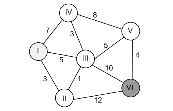
The problem to find a “shortest” path from one vertex to another through a connected graph is of interest in multiple domains, most prominently in the internet, where it is used to find an optimal route for a data packet. The term “shortest” refers here to the minimum cumulative edge cost, which could be physical distance (in a robotic application), delay (in a networking application) or any other metric that is important for a specific application. An example graph with arbitrary edgelengths is shown in Figure 4.2.1.

Figure \(\PageIndex{1}\): A generic path planning problem from vertex I to vertex VI. The shortest path is I-II-III-V-VI with length 13.

4.2.1. Robot embodiment

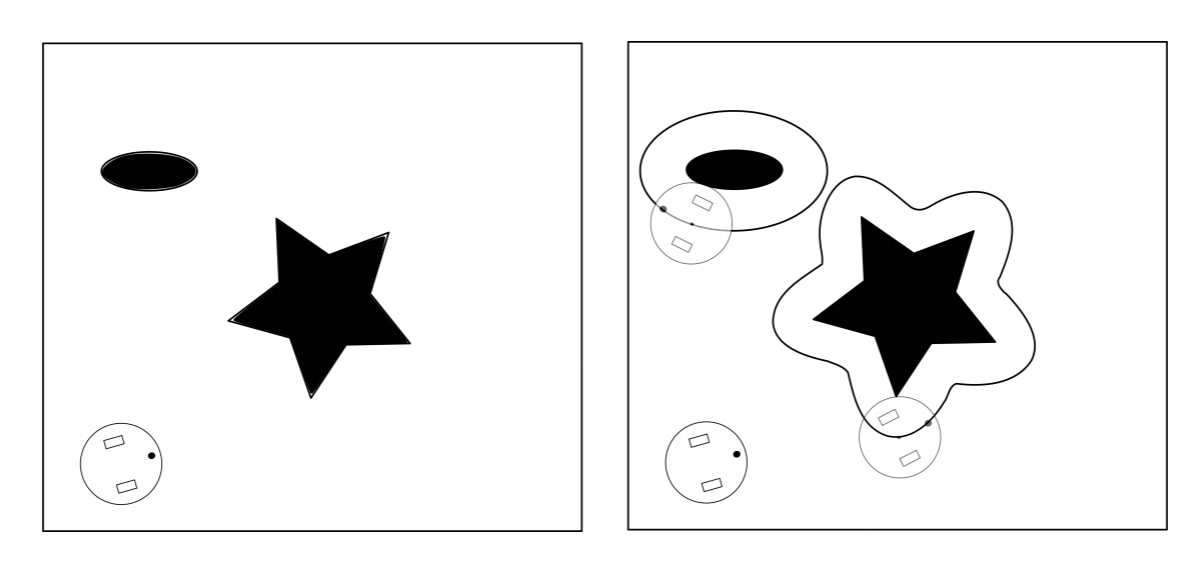
In order to deal with the physical embodiment of the robot, which complicates the path-planning process, the robot is reduced to a point-mass and all the obstacles in the environment are grown by half of the longest extension of the robot from its center. This representation is known as configuration space as it reduces the representation of the robot to its x and y coordinates in the plane. An example is shown in Figure 4.2.2. The configuration space can now either be used as a basis for a grid map or a continuous representation.

Figure \(\PageIndex{2}\): A map with obstacles and its representation in configuration space, which can be obtained by growing each obstacle by the robot’s extension.

4.2.2. Dijkstra’s algorithm

One of the earliest and simplest algorithms is Dijkstra’s algorithm (Dijkstra 1959). Starting from the initial vertex where the path should start, the algorithm marks all direct neighbors of the initial vertex with the cost to get there. It then proceeds from the vertex with the lowest cost to all of its adjacent vertices and marks them with the cost to get to them via itself if this cost is lower. Once all neighbors of a vertex have been checked, the algorithm proceeds to the vertex with the next lowest cost. Once the algorithm reaches the goal vertex, it terminates and the robot can follow the edges pointing towards the lowest edge cost.

In Figure 4.2.1, Dijkstra would first mark nodes II, III and IV with cost 3, 5 and 7 respectively. It would then continue to explore all edges of node II, which so far has the lowest cost. This would lead to the discovery that node III can actually be reached in 3+1 < 5 steps, and node III would be relabeled with cost 4. In order to completely evaluate node II, Dijkstra needs to evaluate the remaining edge before moving on and label node VI with 3 + 12 = 15.

The node with the lowest cost is now node III (4). We can now relabel node VI with 14, which is smaller than 15, and label node V with 4 + 5 = 9, whereas node IV remains at 4 + 3 = 7. Although we have already found two paths to the goal, one of which better than the other, we cannot stop as there still exist nodes with unexplored edges and overall cost lower than 14. Indeed, continuing to explore from node V leads to a shortest path I-II-III-V-VI of cost 13, with no remaining nodes to explore.

As Dijkstra would not stop until there is no node with lower cost than the current cost to the goal, we can be sure that a shortest path will be found if it exists. We can say that the algorithm is complete.

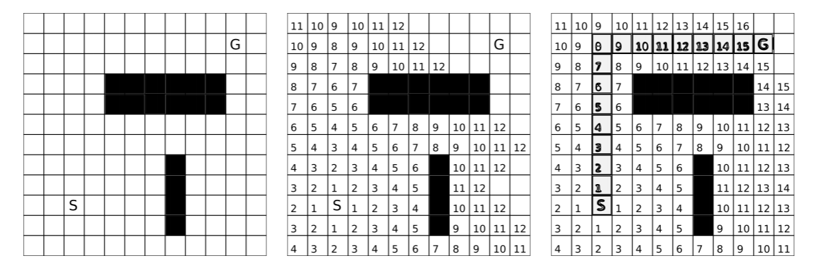
As Dijkstra will always explore nodes with the least overall cost first, the environment is explored comparably to a wave front originating from the start vertex, eventually arriving at the goal. This is of course highly inefficient in particular if Dijkstra is exploring nodes away from the goal. This can be visualized by adding a couple of nodes to the left of node I in Figure 4.2.1. Dijkstra will explore all of these nodes until their cost exceeds the lowest found for the goal. This can also be seen when observing Dijkstra’s algorithm on a grid, as shown in Figure 4.2.3.

Figure \(\PageIndex{3}\): Dijkstra’s algorithm finding a shortest path from ‘S’ to ‘G’ assuming the robot can only travel laterally (not diagonally) with cost one per grid cell. Note the few number of cells that remain unexplored once the shortest path (grey) is found, as Dijkstra would always consider a cell with the lowest path cost first.

4.2.3. A*

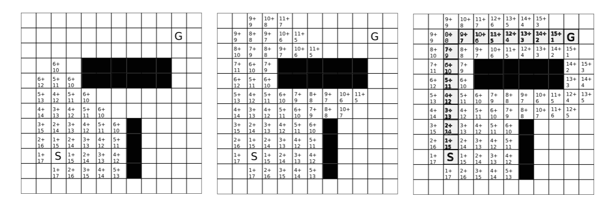
Instead of exploring in all directions, knowledge of an approximate direction of the goal could help avoiding exploring nodes that are obviously wrong to a human observer. Such special knowledge that such an observer has can be encoded using a heuristic function, a fancier word for a “rule of thumb”. For example, we could give priority to nodes that have a lower estimated distance to the goal than others. For this, we would mark every node not only with the actual distance that it took us to get there (as in Dijkstra’s algorithm), but also with the estimated cost “as the crow flies”, for example by calculating the Euclidean distance or the Manhattan distance between the vertex we are looking at and the goal vertex. This algorithm is known as A* (Hart, Nilsson & Raphael 1968). Depending on the environment, A* might accomplish search much faster than Dijkstra’s algorithm, and performs the same in the worst case. This is illustrated in Figure 4.2.4 using the Manhattan distance metric, which does not allow for diagonal movements.

Figure \(\PageIndex{4}\): Finding a shortest path from ‘S’ to ‘G’ assuming the robot can only travel laterally (not diagonally) with cost one per grid cell using the A* algorithm. Much like Dijkstra, A* evaluates only the cell with the lowest cost, but takes an estimate of the remaining distance into account.

An extension of A* that addresses the problem of expensive re-planning when obstacles appear in the path of the robot, is known as D* (Stentz 1994). Unlike A*, D* starts from the goal vertex and has the ability to change the costs of parts of the path that include an obstacle. This allows D* to replan around an obstacle while maintaining most of the already calculated path.

A* and D* become computationally expensive when either the search space is large, e.g., due to a fine-grain resolution required for the task, or the dimensions of the search problem are high, e.g. when planning for an arm with multiple degrees of freedom. Solutions to these problems are provided by samplingbased path planning algorithms that are described further below.