4.3: Sampling-based Path Planning

The previous sections have introduced a series of complete algorithms for the path planning problem, i.e. they will find a solution eventually if it exists. Complete solutions are often unfeasible, however, when the possible state space is large. This is the case for robots with multiple degrees of freedom such as arms. In practice, most algorithms are only resolution complete, i.e., only complete if the resolution is fine-grained enough, as the state-space needs to be somewhat discretized for them to operate (e.g., into a grid) and some solutions might be missed as a function of the resolution of the discretization.

Figure \(\PageIndex{1}\): Counterclockwise: Random exploration of a 2D search space by randomly sampling points and connecting them to the graph until a feasible path between start and goal is found.

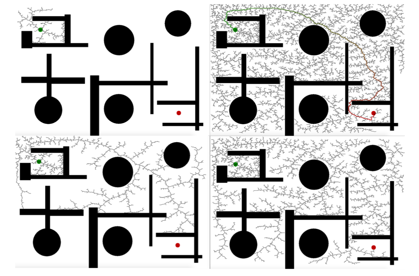
Instead of evaluating all possible solutions or using a noncomplete Jacobian-based inverse kinematic solution, samplingbased planners create possible paths by randomly adding points to a tree until some solution is found or time expires. As the probability to find a path approaches one when time goes to infinity, sampling-based path planners are probabilistic complete. Prominent examples of sampling-based planners are Rapidlyexploring Random Trees (RRT)(LaValle 1998) and Probabilistic Roadmaps(PRM) (Kavraki, Svestka, Latombe & Overmars 1996). An example execution of RRT for an unknown goal, thereby reducing the path-planning problem to a search problem is shown in Figure 4.3.1.

This example illustrates well how a sampling-based planner can quickly explore a large portion of space and refines a solution as time goes on. Whereas RRT can be understood as growing a single tree from a robot’s starting point until one of its branches hits a goal, probabilistic road-maps create a tree by randomly sampling points in the state-space, testing whether they are collision-free, connecting them with neighboring points using paths that reflect the kinematics of a robot, and then using classical graph shortest path algorithms to find shortest paths on the resulting structure. The advantage of this approach is clearly that such a probabilistic roadmap has to be created only once (assuming the environment is not changing) and can then be used for multiple queries. PRMs are therefore a multi-query path-planning algorithm. In contrast, RRT’s are known as single-query path-planning algorithms.

In practice, the boundary between the different historic algorithms has become very diffuse, and single-query and multiquery variants of both RRT and PRM exist. It is important to note that there is no silver bullet algorithm/heuristic and even their parameter-sets are highly problem-specific. We will therefore limit our discussion on useful heuristics that are common to sampling-based planners.

4.3.1. Basic Algorithm

Let X be a d-dimensional state-space. This can either be the robot’s state given in terms of translation and rotations (6 dimensions), a subset thereof, or the joint space with one dimension per possible joint angle. Let G ⊂ X be a d-ball (ddimensional sphere) in the state-space that is considered to be the goal, and t the allowed time. A tree planner proceeds as follows:

Tree=Init(X,start);

WHILE ElapsedTime() < t AND NoGoalFound(G) DO

newpoint = StateToExpandFrom(Tree);

newsegment = CreatePathToTree(newpoint);

IF ChooseToAdd(newsegment) THEN

Tree=Insert(Tree,newsegment);

ENDIF

ENDWHILE

return Tree

This process can be repeated on the resulting tree as long as time allows. This is known as an AnyTime algorithm. Given a suitable distance metric, the cost-to-goal can be stored at each node of the tree (much easier if growing the tree from the goal to start), which allows retrieving the shortest path easily. There are four key points in this algorithm:

1. Finding the next point to add to the tree (or discard) (StateToExpandFrom).
2. Finding out where and how to connect this point to the tree taking into account the robot kinematics (CreatePathToTree).
3. Testing whether this path is suitable, i.e., collision-free.
4. Finding the next point to add.

A prominent method is to pick a random point in the statespace and connect it to the closest existing point in the tree or to the goal. This requires searching all nodes in the tree and calculating their distance to the candidate point. Other approaches put preferences on nodes with fewer out-degrees (those which do not yet have very many connections) and choose a new point within its vicinity. Both approaches make it likely to quickly explore the entire state-space.

If there are constraints imposed on the robot’s path, for example the robot needs to hold a cup and therefore is not supposed to rotate its wrist, this dimension can simply be taken out of the state-space.

Once a possible path is found, this space can be reduced to the ellipsoid that bounds the maximal path-length. This ellipsoid can be constructed by mounting a wire of the maximum path length between start and goal and pushing it outward with a pen. All the area that can be reached with the pen constrained by the wire can contain a point that can possibly lead to a shorter path. This approach is particularly effective when running multiple copies of the same planner in parallel and exchanging the shortest paths once they are found (Otte & Correll 2013).

4.3.2. Connecting Points to the Tree

A new point is classically connected to the closest point already in the tree or to the goal. This can be done by calculating the distance to all points already in the tree. This does not necessarily generate the shortest path, however. A recent improvement has been made by RRT*, which connects the point to the tree in a way that minimizes the overall path length. This can be done by considering all points in the tree within a d-ball (on a 2D map, d = 2, i.e. a circle) from of fixed radius from the point to add and finding the point that minimizes the overall path length to the start.

Adding a point to the tree is also a good time to take into account the specific kinematics of a robot, for example a car. Here, a local planner can be used to generate a suitable trajectory that takes into account the orientation of the vehicle at each point in the tree.

4.3.3. Collision Checking

Efficient algorithms for testing collisions deserve a dedicated section. While the problem is intuitive in configuration-space planning in 2D (the robot reduces to a point) and can be solved using a simple point-in-polygon test, the problem is more involved for manipulators that are subject to self-collision.

As collision checking takes up to 90% of the execution time in the path-planning problem, a successful method to increase computational speed is “lazy collision evaluation”. Instead of checking every point for a possible collision, the algorithm first finds a suitable path. Only then, it checks every segment of this path for collisions. In case some segments are in collision, they are deleted and the algorithm goes on, but keeps the segments of the successful path that were collision-free.