7.3: Line Recognition

Why are lines a useful feature? As you will see next chapter, the key challenge in estimating a robot’s pose is unreliable odometry, in particular when it comes to turning. Here, a simple infrared sensor measuring the distance to a wall can provide the robot with a much better feel for what actually happened. Similarly, if a robot has the ability to track markers in the environment using vision, it gets another estimate on how much it is actually moving. How information from odometry and other sensors can be fused not only to localize the robot, but also to create maps of its environment, will be the focus of the remainder of this book.

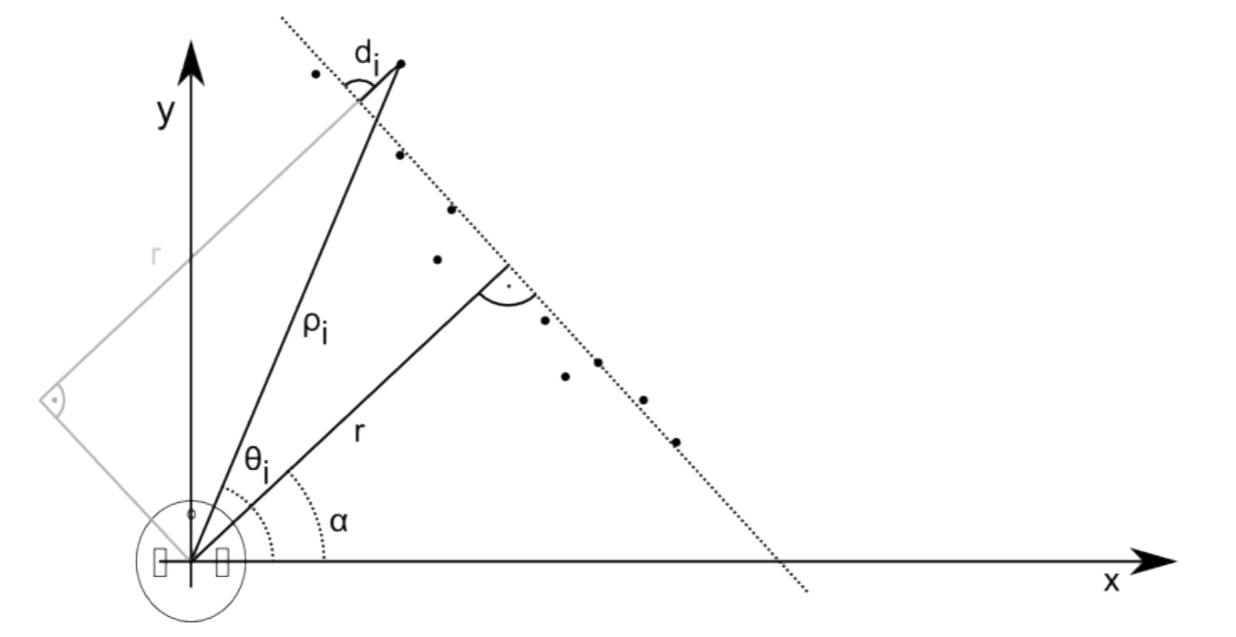
A laser scanner or similar device pointed against a wall will return a suite of N points at position (xi , yi) in the robot’s coordinate system. These points can also be represented in polar coordinates (ρi , θi). We can now imagine a line running through these points that is parametrized with a distance r and an angle α. Here, r is the distance of the robot to the wall and α its angle. As all sensors are noisy, each point will have distance di from the “optimal” line running through the points. These relationships are illustrated in Figure 7.2.1.

7.3.1. Line fitting using least squares

Using simple trigonometry we can now write

\[\rho _{i} \cos(\theta _{i}-\alpha )-r=d_{i}\]

Different line candidates — parametrized by r and α — will have different values for d_i . We can now write an expression for the total error S_r,α as

\[S_{r,\alpha }=\sum_{i=1}^{N}d_{i}^{2}=\sum_{i}^{}(\rho _{i}\cos(\theta _{i}-\alpha )-r)^{2}\]

Figure \(\PageIndex{1}\): A 2D point cloud recorded by a laser-scanner or similar device. A line (dashed) is fitted through the points in a least-square sense.

Here, we square each individual error to account for the fact that a negative error, i.e. a point left of the line, is as bad as a positive error, i.e. a point right of the optimal line. In order to optimize S_r,α, we need to take the partial derivatives with respect to r and α, set them zero, and solve the resulting system of equations for r and α.

\[\frac{∂S}{∂\alpha }=0 \\ \frac{∂S}{∂r}=0\]

Here, the symbol ∂ indicates that we are taking a partial derivative. Solving for r and α is involved, but possible (Siegwart et al. 2011):

\[\alpha =\frac{1}{2}atan\left ( \frac{\frac{1}{N}\sum \rho _{i}^{2}sin2\theta _{i}-\frac{2}{N^{2}}\sum \sum\rho _{i}\rho _{j}cos\theta _{i}sin_{j}}{\frac{1}{N}\sum \rho _{i}^{2}cos2\theta _{i}-\frac{1}{N^{2}}\sum \sum\rho _{i}\rho _{j}cos(\theta _{i}+\theta _{j})} \right )\]

and

\[r=\frac{\sum \rho _{i}cos(\theta _{i}-\alpha )}{N}\]

We can therefore calculate the distance and orientation of a wall captured by our proximity sensors relative to the robot’s positions or the height and orientation of a line in an image based on a collection of points that we believe might belong to a line.

Figure \(\PageIndex{2}\): Split-and-merge algorithm. Initial least-square fit of a line (left). Splitting the data-set at the point with the highest error (after picking a direction) allows fitting two lines with overall lesser error.

This approach is known as the least-square method and can be used to fit data to any parametric model. The general approach is to describe the fit between the data and the model in terms of an error. The best fit will minimize this function, which will therefore have a zero derivative at this point. If the result cannot be obtained analytically as in this example, numerical methods have to be used to find the best fit that minimizes the quadratic error.

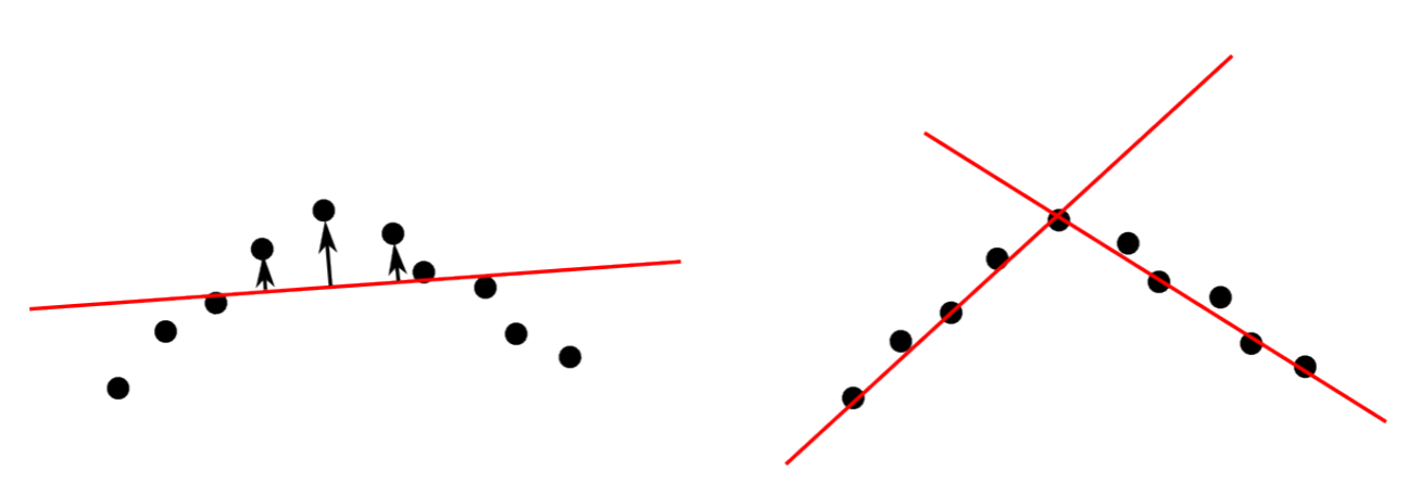
7.3.2. Split-and-merge algorithm

A key problem with this approach is that it is often unclear how many lines there are and where a line starts and where it ends. Looking through the camera, for example, we will see vertical lines corresponding to wall corners and horizontal ones that correspond to wall-floor intersections and the horizon; using a distance sensor, the robot might detect a corner. We therefore need an algorithm that can separate point clouds into multiple lines. One possible approach is to find the outlier with the strongest deviation from a fitted line and split the line at this point. This is illustrated in Figure 7.3.2. This can be done iteratively until each line has no outliers above a certain threshold.

Figure \(\PageIndex{3}\): Random Sample and Consensus (RANSAC). Random lines are evaluated by counting the number of points close by (”inliers”), darker lines are better fits.

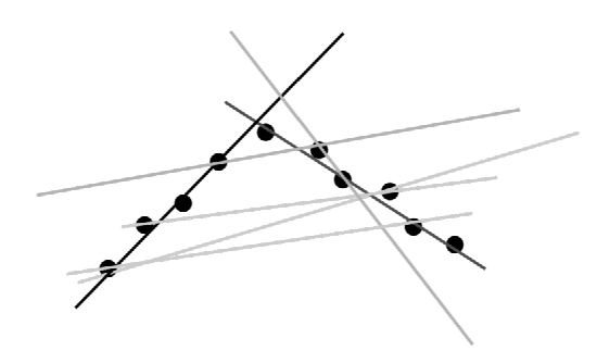
7.3.3. RANSAC: Random Sample and Consensus

If the number of “outliers” is large, a least square fit will generate poor results as it will generate the “best” fit that accomodates both “inliers” and “outliers”. Also, split-and-merge algorithms will fail as they are extremely susceptive to noise: depending on the actual parameters every outlier will split a potential line into two. A solution to this problem is to randomly sample possible lines and keep those that satisfy a certain desired quality given by the number of points being somewhat close to the best fit. This is illustrated in Figure 7.3.3, with darker lines corresponding to better fits. RANSAC usually requires two parameters, namely the number of points required to consider a line to be a valid fit, and the maximum di from a line to consider a point an inlier and not an outlier. The algorithm proceeds as follows: select two random points from the set and connect them with a line. Grow this line by di in both directions and count the number of inliers. Repeat this until one or more lines that have sufficient number of inliers are found, or a maximum number of iterations is reached.

The RANSAC algorithm is fairly easy to understand in the line fitting application, but can be used to fit arbitrary parametric models to any-dimensional data. Here, its main strength is to cope with noisy data.

Given that RANSAC is random, finding a really good fit will take quite some time. Therefore, RANSAC is usually used only as a first step to get an initial estimate, which can then be improved by some kind of local optimization, such as least-squares, e.g.

7.3.4. The Hough Transform

The Hough transform can best be understood as a voting scheme to guess the parametrization of a feature such as a line, circle or other curve (Duda & Hart 1972). For example, a line might be represented by y = mx+c, where m and c are the gradient and offset. A point in this parameter space (or “Hough-space”) then corresponds to a specific line in x−y-space (or “image-space”). The Hough-transform now proceeds as follows: for every pixel in the image that could be part of a line, e.g., white pixels in a thresholded image after Sobel filtering, construct all possible lines that intersect this point. (Drawing an image of this would look like a star). Each of these lines has a specifc m and c associated with it, for which we can add a white dot in Houghspace. Continuing to do this for every pixel of a line in an image will yield many m − c pair, but only one that is common among all those pixels of the line in the image: the actual m−c parameters of this line. Thinking about the number of times a point was highlighted in Hough-space as brightness, will turn a line in image space into a bright spot in Hough-space (and the other way round). In practice, a polar representation is chosen for lines. This is shown in Figure 7.4.1. The Hough transform also generalizes to other parametrization such as circles.