12.3: RGB-D Mapping

Last updated
Save as PDF

Page ID: 14846

\( \newcommand{\vecs}[1]{\overset { \scriptstyle \rightharpoonup} {\mathbf{#1}} } \) \( \newcommand{\vecd}[1]{\overset{-\!-\!\rightharpoonup}{\vphantom{a}\smash {#1}}} \)\(\newcommand{\id}{\mathrm{id}}\) \( \newcommand{\Span}{\mathrm{span}}\) \( \newcommand{\kernel}{\mathrm{null}\,}\) \( \newcommand{\range}{\mathrm{range}\,}\) \( \newcommand{\RealPart}{\mathrm{Re}}\) \( \newcommand{\ImaginaryPart}{\mathrm{Im}}\) \( \newcommand{\Argument}{\mathrm{Arg}}\) \( \newcommand{\norm}[1]{\| #1 \|}\) \( \newcommand{\inner}[2]{\langle #1, #2 \rangle}\) \( \newcommand{\Span}{\mathrm{span}}\) \(\newcommand{\id}{\mathrm{id}}\) \( \newcommand{\Span}{\mathrm{span}}\) \( \newcommand{\kernel}{\mathrm{null}\,}\) \( \newcommand{\range}{\mathrm{range}\,}\) \( \newcommand{\RealPart}{\mathrm{Re}}\) \( \newcommand{\ImaginaryPart}{\mathrm{Im}}\) \( \newcommand{\Argument}{\mathrm{Arg}}\) \( \newcommand{\norm}[1]{\| #1 \|}\) \( \newcommand{\inner}[2]{\langle #1, #2 \rangle}\) \( \newcommand{\Span}{\mathrm{span}}\)\(\newcommand{\AA}{\unicode[.8,0]{x212B}}\)

The ICP algorithm can be used to stitch consecutive range images together to create a 3D map of the environment (Henry, Krainin, Herbst, Ren & Fox 2010). Together with RGB information, it is possible to create complete 3D walk throughs of an environment. An example of such a walk through using the method described in (Whelan, Johannsson, Kaess, Leonard & McDonald 2013) is shown in Figure 12.3.1. A problem with ICP is that errors in each transformation propagate making maps created using this method as odd as maps created by simple odometry. Here, the SLAM algorithm can be used to correct previous errors once a loop closure is detected.

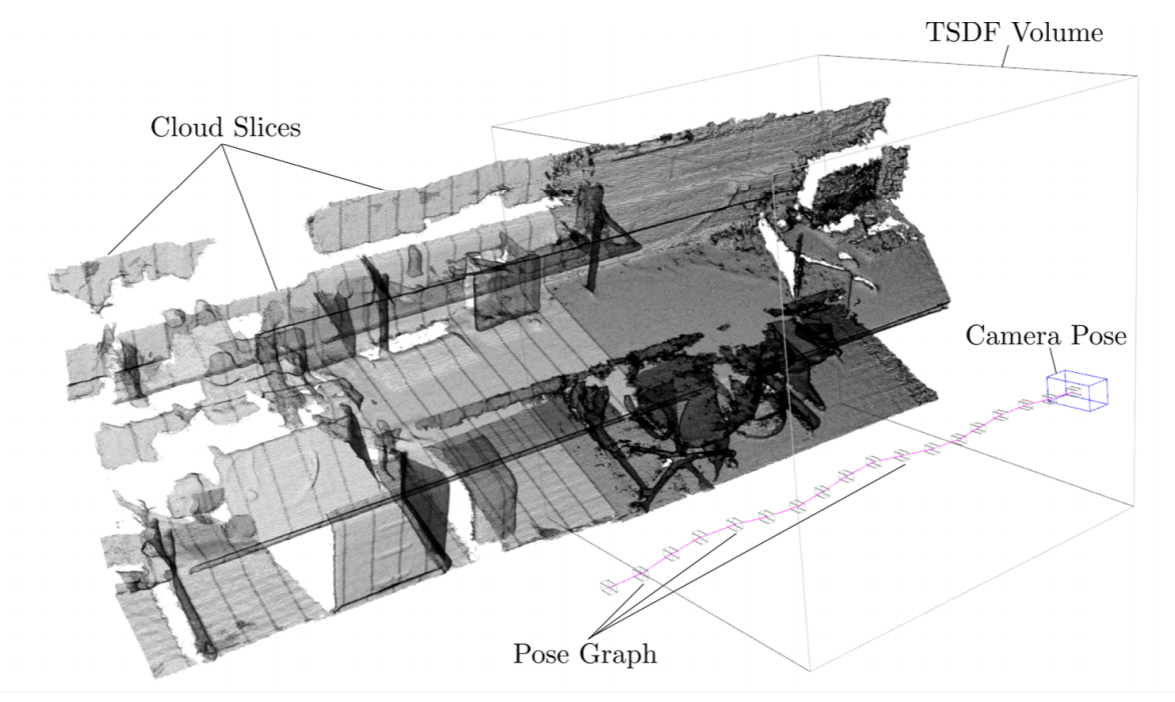
Figure \(\PageIndex{1}\): Fused point cloud data from a walk trough of an office environment using “Kintinious”. Picture courtesy of John Leonard.

The intuition behind SLAM is to consider each transformation between consecutive snapshots as a spring with variable stiffness. Whenever the robot returns to a previously seen location, i.e., a loop-closure has been determined, additional constraints are introduced and the collection of snapshots connected by springs become a mesh. Everytime the robot then re-observes a transformation between any of the snapshots, it can “stiffen” the spring connecting the two. As all of the snapshots are connected, this new constraints propagates through the network and literally pull each snapshots in place.

RGB-D Mapping uses a variant of ICP that is enhanced by SIFT features for point selection and matching. Maps are build incrementally. SIFT features, and their spatial relationship, are used for detecting loop closures. Once a loop closure is detected, an additional constraint is added to the pose graph and a SLAM-like optimization algorithm corrects the pose of all previous observations.

As ICP only works when both point clouds are already closely aligned, which might not be the case for a fast moving robot with a relatively noisy sensor (the XBox Kinect has an error of 3cm for a few meters of range vs. millimeters in laser range scanners), RGB-D Mapping uses RANSAC to find an initial transformation. Here, RANSAC works as for line fitting: it keeps guessing possible transformations for 3 pairs of SIFT feature points and then counts the number of inliers when matching the two point clouds, one of which being transformed using the random guess.