2.2: Interpolation of Bivariate Functions

This section considers interpolation of bivariate functions, i.e., functions of two variables. Following the approach taken in constructing interpolants for univariate functions, we first discretize the domain into smaller regions, namely triangles. The process of decomposing a domain, \(D \subset \mathbb{R}^{2}\), into a set of non-overlapping triangles \(\left\{R_{i}\right\}_{i=1}^{N}\) is called triangulation. An example of triangulation is shown in Figure 2.15. By construction, the triangles fill the domain in the sense that \[D=\bigcup_{i=1}^{N} \bar{R}_{i},\] where \(\cup\) denotes the union of the triangles. The triangulation is characterized by the size \(h\), which is the maximum diameter of the circumscribed circles for the triangles.

Figure 2.16: Function \(f(x, y)=\sin (\pi x) \sin (\pi y)\)

For the next two examples, we consider interpolation of bivariate function \[f(x, y)=\sin (\pi x) \sin (\pi y), \quad(x, y) \in[0,1]^{2} .\] The function is shown in Figure \(\underline{2.16}\).

Example 2.2.1 Piecewise-constant, centroid

The first interpolant approximates function \(f\) by a piecewise-constant function. To construct a constant function on \(R\), we need just one interpolation point, i.e., \(M=1\). Let us choose the centroid of the triangle to be the interpolation point, \[\overline{\boldsymbol{x}}^{\mathbf{1}}=\frac{1}{3}\left(\boldsymbol{x}_{1}+\boldsymbol{x}_{2}+\boldsymbol{x}_{3}\right) .\] The constant interpolant is given by \[\mathcal{I} f(\boldsymbol{x})=f\left(\overline{\boldsymbol{x}}^{1}\right), \quad \forall \boldsymbol{x} \in R .\] An example of piecewise-constant interpolant is shown in Figure 2.17(a). Note that the interpolant is discontinuous across the triangle interfaces in general.

The error in the interpolant is bounded by \[e \leq h \max _{\boldsymbol{x} \in R}\|\nabla f(\boldsymbol{x})\|_{2},\] where \(\|\nabla f(\boldsymbol{x})\|_{2}\) is the two-norm of the gradient, i.e. \[\|\nabla f\|_{2}=\sqrt{\left(\frac{\partial f}{\partial x}\right)^{2}+\left(\frac{\partial f}{\partial y}\right)^{2}} .\] The interpolant is first-order accurate and is exact if \(f\) is constant. Figure 2.17(b) confirms the \(h^{1}\) convergence of the error.

Example 2.2.2 Piecewise-linear, vertices

This interpolant approximates function \(f\) by a piecewise-linear function. Note that a linear function in two dimension is characterized by three parameters. Thus, to construct a linear function on a

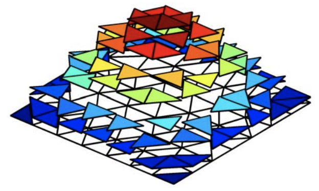
(a) interpolant

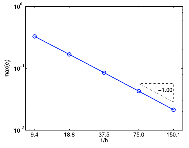
(b) error

Figure 2.17: Piecewise-constant interpolation

triangular patch \(R\), we need to choose three interpolation points, i.e., \(M=3\). Let us choose the vertices of the triangle to be the interpolation point, \[\overline{\boldsymbol{x}}^{1}=\boldsymbol{x}_{1}, \quad \overline{\boldsymbol{x}}^{2}=\boldsymbol{x}_{2}, \quad \text { and } \quad \overline{\boldsymbol{x}}^{3}=\boldsymbol{x}_{3}\] The linear interpolant is of the form \[(\mathcal{I} f)(\boldsymbol{x})=a+b x+c y\] To find the three parameters, \(a, b\), and \(c\), we impose the constraint that the interpolant matches the function value at the three vertices. The constraint results in a system of three linear equations \[\begin{aligned} &(\mathcal{I} f)\left(\overline{\boldsymbol{x}}^{1}\right)=a+b \bar{x}^{1}+c \bar{y}^{1}=f\left(\overline{\boldsymbol{x}}^{1}\right) \\ &(\mathcal{I} f)\left(\overline{\boldsymbol{x}}^{2}\right)=a+b \bar{x}^{2}+c \bar{y}^{2}=f\left(\overline{\boldsymbol{x}}^{2}\right) \\ &(\mathcal{I} f)\left(\overline{\boldsymbol{x}}^{3}\right)=a+b \bar{x}^{3}+c \bar{y}^{3}=f\left(\overline{\boldsymbol{x}}^{3}\right) \end{aligned}\] which can be also be written concisely in the matrix form \[\left(\begin{array}{lll} 1 & \bar{x}^{1} & \bar{y}^{1} \\ 1 & \bar{x}^{2} & \bar{y}^{2} \\ 1 & \bar{x}^{3} & \bar{y}^{3} \end{array}\right)\left(\begin{array}{l} a \\ b \\ c \end{array}\right)=\left(\begin{array}{l} f\left(\bar{x}^{1}\right) \\ f\left(\bar{x}^{2}\right) \\ f\left(\bar{x}^{3}\right) \end{array}\right)\] The resulting interpolant is shown in Figure \(2.18(\mathrm{a})\). Unlike the piecewise-constant interpolant, the piecewise-linear interpolant is continuous across the triangle interfaces.

The approach for constructing the linear interpolation requires solving a system of three linear equations. An alternative more efficient approach is to consider a different form of the interpolant. Namely, we consider the form \[(\mathcal{I} f)(\boldsymbol{x})=f\left(\bar{x}^{1}\right)+b^{\prime}\left(x-\bar{x}^{1}\right)+c^{\prime}\left(y-\bar{y}^{1}\right)\]

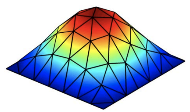
(a) interpolant

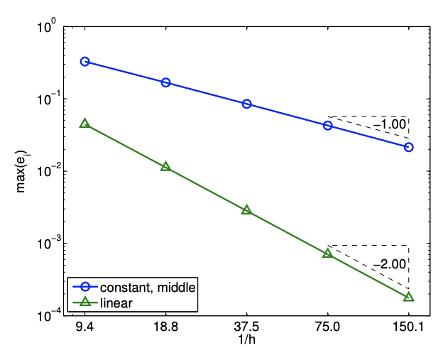
(b) error

Figure 2.18: Piecewise-linear interpolation

Note that the interpolant is still linear, but it already satisfies the interpolation condition at \(\left(\overline{\boldsymbol{x}}^{1}, f\left(\overline{\boldsymbol{x}}^{1}\right)\right)\) because \[(\mathcal{I} f)\left(\overline{\boldsymbol{x}}^{1}\right)=f\left(\overline{\boldsymbol{x}}^{1}\right)+b^{\prime}\left(\bar{x}^{1}-\bar{x}^{1}\right)+c^{\prime}\left(\bar{y}^{1}-\bar{y}^{1}\right)=f\left(\overline{\boldsymbol{x}}^{1}\right)\] Thus, our task has been simplified to that of finding the two coefficients \(b^{\prime}\) and \(c^{\prime}\), as oppose to the three coefficients \(a, b\), and \(c\). We choose the two coefficients such that the interpolant satisfies the interpolaion condition at \(\overline{\boldsymbol{x}}^{2}\) and \(\overline{\boldsymbol{x}}^{3}\), i.e. \[\begin{aligned} &(\mathcal{I} f)\left(\bar{x}^{2}\right)=f\left(\bar{x}^{1}\right)+b^{\prime}\left(\bar{x}^{2}-\bar{x}^{1}\right)+c^{\prime}\left(\bar{y}^{2}-\bar{y}^{1}\right)=f\left(\bar{x}^{2}\right) \\ &(\mathcal{I} f)\left(\bar{x}^{3}\right)=f\left(\bar{x}^{1}\right)+b^{\prime}\left(\bar{x}^{3}-\bar{x}^{1}\right)+c^{\prime}\left(\bar{y}^{3}-\bar{y}^{1}\right)=f\left(\bar{x}^{3}\right) \end{aligned}\] Or, more compactly, we can write the equations in matrix form as \[\left(\begin{array}{cc} \bar{x}^{2}-\bar{x}^{1} & \bar{y}^{2}-\bar{y}^{1} \\ \bar{x}^{3}-\bar{x}^{1} & \bar{y}^{3}-\bar{y}^{1} \end{array}\right)\left(\begin{array}{c} b^{\prime} \\ c^{\prime} \end{array}\right)=\left(\begin{array}{c} f\left(\overline{\boldsymbol{x}}^{2}\right)-f\left(\overline{\boldsymbol{x}}^{1}\right) \\ f\left(\overline{\boldsymbol{x}}^{3}\right)-f\left(\overline{\boldsymbol{x}}^{1}\right) \end{array}\right)\] With some arithmetics, we can find an explicit form of the coefficients, \[\begin{aligned} b^{\prime} &=\frac{1}{A}\left[\left(f\left(\bar{x}^{2}\right)-f\left(\bar{x}^{1}\right)\right)\left(\bar{y}^{3}-\bar{y}^{1}\right)-\left(f\left(\bar{x}^{3}\right)-f\left(\bar{x}^{1}\right)\right)\left(\bar{y}^{2}-\bar{y}^{1}\right)\right] \\ c^{\prime} &=\frac{1}{A}\left[\left(f\left(\bar{x}^{3}\right)-f\left(\bar{x}^{1}\right)\right)\left(\bar{x}^{2}-\bar{x}^{1}\right)-\left(f\left(\bar{x}^{2}\right)-f\left(\bar{x}^{1}\right)\right)\left(\bar{x}^{3}-\bar{x}^{1}\right)\right] \end{aligned}\] with \[A=\left(\bar{x}^{2}-\bar{x}^{1}\right)\left(\bar{y}^{3}-\bar{y}^{1}\right)-\left(\bar{x}^{3}-\bar{x}^{1}\right)\left(\bar{y}^{2}-\bar{y}^{1}\right)\] Note that \(A\) is twice the area of the triangle. It is important to note that this second form of the linear interpolant is identical to the first form; the interpolant is just expressed in a different form. The error in the interpolant is governed by the Hessian of the function, i.e. \[e \leq C h^{2}\left\|\nabla^{2} f\right\|_{F},\] where \(\left\|\nabla^{2} f\right\|_{F}\) is the Frobenius norm of the Hessian matrix, i.e. \[\left\|\nabla^{2} f\right\|_{F}=\sqrt{\left(\frac{\partial^{2} f}{\partial x^{2}}\right)^{2}+\left(\frac{\partial^{2} f}{\partial y^{2}}\right)^{2}+2\left(\frac{\partial^{2} f}{\partial x \partial y}\right)^{2}} .\] Thus, the piecewise-linear interpolant is second-order accurate and is exact if \(f\) is linear. The convergence result shown in Figure 2.18(b) confirms the \(h^{2}\) convergence of the error.