3.1: Differentiation of Univariate Functions

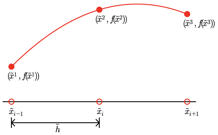
Our objective is to approximate the value of the first derivative, \(f^{\prime}\), for some arbitrary univariate function \(f\). In particular, we assume the values of the function is provided at a set of uniformly spaced points \({ }^{1}\) as shown in Figure 3.1. The spacing between any two function evaluation points is denoted by \(\tilde{h}\).

Our approach to estimating the derivative is to approximate function \(f\) by its interpolant If constructed from the sampled points and then differentiate the interpolant. Note that the interpolation rules based on piecewise-constant representation do not provide meaningful results, as they cannot represent nonzero derivatives. Thus, we will only consider linear and higher order interpolation rules.

To construct an interpolant \(\mathcal{I} f\) in the neighborhood of \(\tilde{x}_{i}\), we can first choose \(M\) interpolation points, \(\tilde{x}_{j}, j=s(i), \ldots, s(i)+M-1\) in the neighborhood of \(\tilde{x}_{i}\), where \(s(i)\) is the global function evaluation index of the left most interpolation point. Then, we can construct an interpolant \(\mathcal{I} f\) from the pairs \(\left(\tilde{x}_{j}, \mathcal{I} f\left(\tilde{x}_{j}\right)\right), j=s(i), \ldots, s(i)+M-1\); note that \(\mathcal{I} f\) depends linearly on the

\({ }^{1}\) The uniform spacing is not necessary, but it simplifies the analysis

Figure 3.1: Stencil for one-dimensional numerical differentiation.

function values, as we know from the Lagrange basis construction. As a result, the derivative of the interpolant is also a linear function of \(f\left(\tilde{x}_{j}\right), j=s(i), \ldots, s(i)+M-1\). Specifically, our numerical approximation to the derivative, \(f_{h}^{\prime}\left(\tilde{x}_{i}\right)\), is of the form \[f_{h}^{\prime}\left(\tilde{x}_{i}\right) \approx \sum_{j=s(i)}^{s(i)+M-1} \omega_{j}(i) f\left(\tilde{x}_{j}\right),\] where \(\omega_{j}(i), j=1, \ldots, M\), are weights that are dependent on the choice of interpolant.

These formulas for approximating the derivative are called finite difference formulas. In the context of numerical differentiation, the set of function evaluation points used to approximate the derivative at \(\tilde{x}_{i}\) is called numerical stencil. A scheme requiring \(M\) points to approximate the derivative has an \(M\)-point stencil. The scheme is said to be one-sided, if the derivative estimate only involves the function values for either \(\tilde{x} \geq \tilde{x}_{i}\) or \(\tilde{x} \leq \tilde{x}_{i}\). The computational cost of numerical differentiation is related to the size of stencil, \(M\).

Throughout this chapter, we assess the quality of finite difference formulas in terms of the error \[e \equiv\left|f^{\prime}\left(\tilde{x}_{i}\right)-f_{h}^{\prime}\left(\tilde{x}_{i}\right)\right| .\] Specifically, we are interested in analyzing the behavior of the error as our discretization is refined, i.e., as \(\tilde{h}\) decreases. Note that, because the interpolant, \(\mathcal{I} f\), from which \(f_{h}^{\prime}\left(\tilde{x}_{i}\right)\) is constructed approaches \(f\) as \(\tilde{h} \rightarrow 0\) for smooth functions, we also expect \(f_{h}^{\prime}\left(\tilde{x}_{i}\right)\) to approach \(f^{\prime}\left(\tilde{x}_{i}\right)\) as \(\tilde{h} \rightarrow 0\). Thus, our goal is not just to verify that \(f^{\prime}\left(\tilde{x}_{i}\right)\) approaches \(f\left(\tilde{x}_{i}\right)\), but also to quantify how fast it converges to the true value.

Let us provide a few examples of the differentiation rules.

Example 3.1.1 forward difference

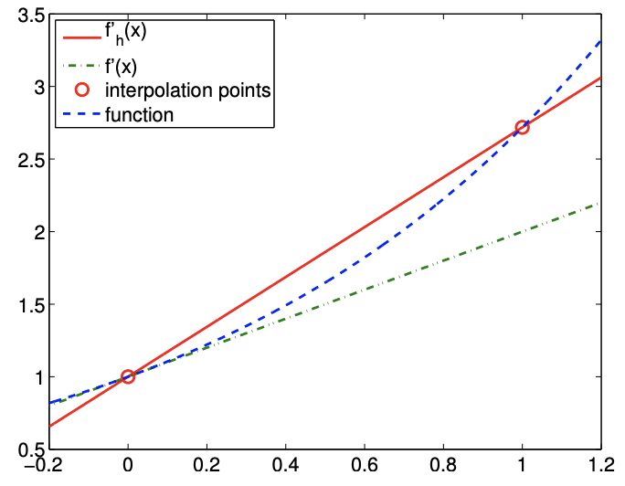
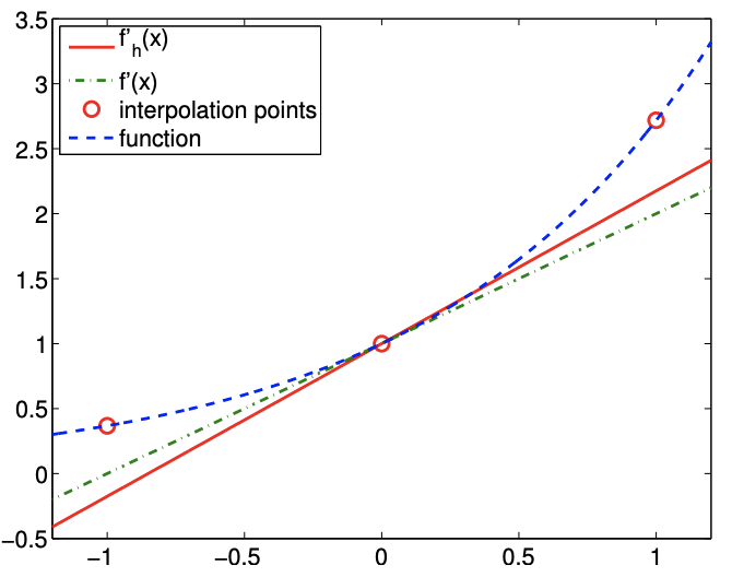
The first example is based on the linear interpolation. To estimate the derivative at \(\tilde{x}_{i}\), let us first construct the linear interpolant over segment \(\left[\tilde{x}_{i}, \tilde{x}_{i+1}\right]\). Substituting the interpolation points \(\bar{x}^{1}=\tilde{x}_{i}\) and \(\bar{x}^{2}=\tilde{x}_{i+1}\) into the expression for linear interpolant, Eq. (2.1), we obtain \[(\mathcal{I} f)(x)=f\left(\tilde{x}_{i}\right)+\frac{1}{\tilde{h}}\left(f\left(\tilde{x}_{i+1}\right)-f\left(\tilde{x}_{i}\right)\right)\left(x-\tilde{x}_{i}\right) .\] The derivative of the interpolant evaluated at \(x=\tilde{x}_{i}\) (approaching from \(x>\tilde{x}_{i}\) ) is \[f_{h}^{\prime}\left(\tilde{x}_{i}\right)=(\mathcal{I} f)^{\prime}\left(\tilde{x}_{i}\right)=\frac{1}{\tilde{h}}\left(f\left(\tilde{x}_{i+1}\right)-f\left(\tilde{x}_{i}\right)\right) .\] The forward difference scheme has a one-sided, 2-point stencil. The differentiation rule applied to \(f(x)=\exp (x)\) about \(x=0\) is shown in Figure 3.2(a). Note that the linear interpolant matches the function at \(\tilde{x}_{i}\) and \(\tilde{x}_{i}+\tilde{h}\) and approximates derivative at \(x=0\).

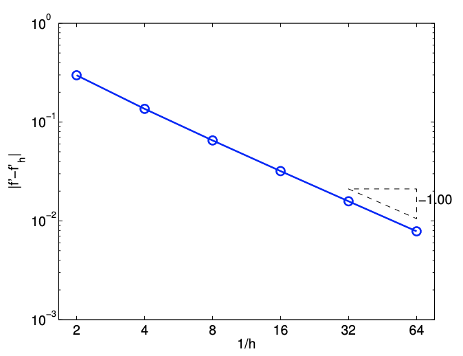
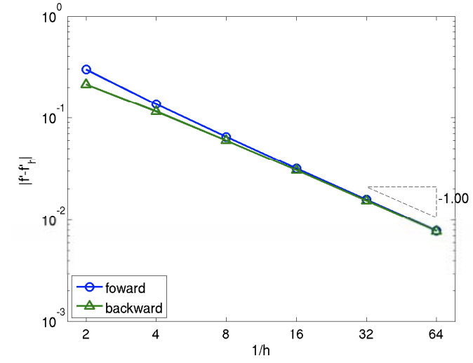
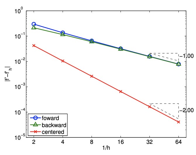
The error in the derivative is bounded by \[e_{i}=\left|f^{\prime}\left(\tilde{x}_{i}\right)-f_{h}^{\prime}\left(\tilde{x}_{i}\right)\right| \leq \frac{\tilde{h}}{2} \max _{x \in\left[\tilde{x}_{i}, \tilde{x}_{i+1}\right]}\left|f^{\prime \prime}(x)\right| .\] The convergence plot in Figure \(\underline{3.2(\mathrm{~b})}\) of the error with respect to \(h\) confirms the first-order convergence of the scheme.

(a) differentiation

(b) error

Figure 3.2: Forward difference.

Proof

The proof of the error bound follows from Taylor expansion. Recall, assuming \(f^{\prime \prime}(x)\) is bounded in \(\left[\tilde{x}_{i}, \tilde{x}_{i+1}\right]\), \[f\left(\tilde{x}_{i+1}\right)=f\left(\tilde{x}_{i}+\tilde{h}\right)=f\left(\tilde{x}_{i}\right)+f^{\prime}\left(\tilde{x}_{i}\right) \tilde{h}+\frac{1}{2} f^{\prime \prime}(\xi) \tilde{h}^{2},\] for some \(\xi \in\left[\tilde{x}_{i}, \tilde{x}_{i+1}\right]\). The derivative of the interpolant evaluated at \(x=\tilde{x}_{i}\) can be expressed as \[(\mathcal{I} f)^{\prime}\left(\tilde{x}_{i}\right)=\frac{1}{\tilde{h}}\left(f\left(\tilde{x}_{i}\right)+f^{\prime}\left(\tilde{x}_{i}\right) \tilde{h}+\frac{1}{2} f^{\prime \prime}(\xi) \tilde{h}^{2}-f\left(\tilde{x}_{i}\right)\right)=f^{\prime}\left(\tilde{x}_{i}\right)+\frac{1}{2} f^{\prime \prime}(\xi) \tilde{h},\] and the error in the derivative is \[\left|f^{\prime}\left(\tilde{x}_{i}\right)-(\mathcal{I} f)^{\prime}\left(\tilde{x}_{i}\right)\right|=\left|\frac{1}{2} f^{\prime \prime}(\xi) \tilde{h}\right| \leq \frac{1}{2} \tilde{h} \max _{x \in\left[\tilde{x}_{i}, \tilde{x}_{i+1}\right]}\left|f^{\prime \prime}(x)\right| .\]

Example 3.1.2 backward difference

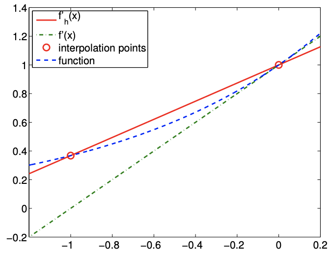
The second example is also based on the piecewise linear interpolation; however, instead of constructing the interpolant over segment \(\left[\tilde{x}_{i}, \tilde{x}_{i+1}\right]\), we construct the interpolant over segment \(\left[\tilde{x}_{i-1}, \tilde{x}_{i}\right]\). Substituting the interpolation points \(\bar{x}^{1}=\tilde{x}_{i-1}\) and \(\bar{x}^{2}=\tilde{x}_{i}\) into the linear interpolant expression, Eq. (2.1), we obtain \[(\mathcal{I} f)(x)=f\left(\tilde{x}_{i-1}\right)+\frac{1}{\tilde{h}}\left(f\left(\tilde{x}_{i}\right)-f\left(\tilde{x}_{i-1}\right)\right)\left(x-\tilde{x}_{i-1}\right)\] The derivative of the interpolant evaluated at \(x=\tilde{x}_{i}\left(\right.\) approaching from \(\left.x<\tilde{x}_{i}\right)\) is \[f_{h}^{\prime}\left(\tilde{x}_{i}\right)=(\mathcal{I} f)^{\prime}\left(\tilde{x}_{i}\right)=\frac{1}{\tilde{h}}\left(f\left(\tilde{x}_{i}\right)-f\left(\tilde{x}_{i-1}\right)\right)\]

(a) differentiation

(b) error

Figure 3.3: Backward difference.

The backward difference scheme has a one-sided, 2-point stencil. The differentiation rule applied to \(f(x)=\exp (x)\) about \(x=0\) is shown in Figure 3.3(a). The construction is similar to that of the forward difference, except that the interpolant matches the function at \(\tilde{x}_{i}-\tilde{h}\) and \(\tilde{x}_{i}\).

The error in the derivative is bounded by \[e_{i}=\left|f^{\prime}\left(\tilde{x}_{i}\right)-f_{h}^{\prime}\left(\tilde{x}_{i}\right)\right| \leq \frac{\tilde{h}}{2} \max _{x \in\left[\tilde{x}_{i-1}, \tilde{x}_{i}\right]}\left|f^{\prime \prime}(x)\right| .\] The proof is similar to the proof for the error bound of the forward difference formula. The convergence plot for \(f(x)=\exp (x)\) is shown in Figure 3.3(b).

Example 3.1.3 centered difference

To develop a more accurate estimate of the derivative at \(\tilde{x}_{i}\), let us construct a quadratic interpolant over segment \(\left[\tilde{x}_{i-1}, \tilde{x}_{i+1}\right]\) using the function values at \(\tilde{x}_{i-1}, \tilde{x}_{i}\), and \(\tilde{x}_{i+1}\), and then differentiate the interpolant. To form the interpolant, we first construct the quadratic Lagrange basis functions on \(\left[\tilde{x}_{i-1}, \tilde{x}_{i+1}\right]\) using the interpolation points \(\bar{x}^{1}=\tilde{x}_{i-1}, \bar{x}^{2}=\tilde{x}_{i}\), and \(\bar{x}^{3}=\tilde{x}_{i+1}\), i.e. \[\begin{gathered} \phi_{1}(x)=\frac{\left(x-\bar{x}^{2}\right)\left(x-\bar{x}^{3}\right)}{\left(\bar{x}^{1}-\bar{x}^{2}\right)\left(\bar{x}^{1}-\bar{x}^{3}\right)}=\frac{\left(x-\tilde{x}_{i}\right)\left(x-\tilde{x}_{i+1}\right)}{\left(\tilde{x}_{i-1}-\tilde{x}_{i}\right)\left(\tilde{x}_{i-1}-\tilde{x}_{i+1}\right)}=\frac{1}{2 \tilde{h}^{2}}\left(x-\tilde{x}_{i}\right)\left(x-\tilde{x}_{i+1}\right) \\ \phi_{2}(x)=\frac{\left(x-\bar{x}^{1}\right)\left(x-\bar{x}^{3}\right)}{\left(\bar{x}^{2}-\bar{x}^{1}\right)\left(\bar{x}^{2}-\bar{x}^{3}\right)}=\frac{\left(x-\tilde{x}_{i-1}\right)\left(x-\tilde{x}_{i+1}\right)}{\left(\tilde{x}_{i}-\tilde{x}_{i-1}\right)\left(\tilde{x}_{i}-\tilde{x}_{i+1}\right)}=-\frac{1}{\tilde{h}^{2}}\left(x-\tilde{x}_{i}\right)\left(x-\tilde{x}_{i+1}\right), \\ \phi_{3}(x)=\frac{\left(x-\bar{x}^{1}\right)\left(x-\bar{x}^{2}\right)}{\left(\bar{x}^{3}-\bar{x}^{1}\right)\left(\bar{x}^{3}-\bar{x}^{2}\right)}=\frac{\left(x-\tilde{x}_{i-1}\right)\left(x-\tilde{x}_{i}\right)}{\left(\tilde{x}_{i+1}-\tilde{x}_{i-1}\right)\left(\tilde{x}_{i+1}-\tilde{x}_{i}\right)}=\frac{1}{2 \tilde{h}^{2}}\left(x-\tilde{x}_{i-1}\right)\left(x-\tilde{x}_{i}\right) \end{gathered}\] where \(\tilde{h}=\tilde{x}_{i+1}-\tilde{x}_{i}=\tilde{x}_{i}-\tilde{x}_{i-1} \cdot^{2}\) Substitution of the basis functions into the expression for a

\({ }^{2}\) Note that, for the quadratic interpolant, \(\tilde{h}\) is half of the \(h\) defined in the previous chapter based on the length of the segment.

(a) differentiation

(b) error

Figure 3.4: Centered difference.

quadratic interpolant, Eq. (2.4), yields \[\begin{aligned} (\mathcal{I} f)(x)=& f\left(\bar{x}^{1}\right) \phi_{1}(x)+f\left(\bar{x}^{2}\right) \phi_{2}(x)+f\left(\bar{x}^{3}\right) \phi_{3}(x) \\ =& \frac{1}{2 \tilde{h}^{2}} f\left(\tilde{x}_{i-1}\right)\left(x-\tilde{x}_{i}\right)\left(x-\tilde{x}_{i+1}\right)-\frac{1}{\tilde{h}^{2}} f\left(\tilde{x}_{i}\right)\left(x-\tilde{x}_{i-1}\right)\left(x-\tilde{x}_{i+1}\right) \\ &+\frac{1}{2 \tilde{h}^{2}} f\left(\tilde{x}_{i+1}\right)\left(x-\tilde{x}_{i-1}\right)\left(x-\tilde{x}_{i}\right) \end{aligned}\] Differentiation of the interpolant yields

\((\mathcal{I} f)^{\prime}(x)=\frac{1}{2 \tilde{h}^{2}} f\left(\tilde{x}_{i-1}\right)\left(2 x-\tilde{x}_{i}-\tilde{x}_{i+1}\right)-\frac{1}{\tilde{h}^{2}} f\left(\tilde{x}_{i}\right)\left(2 x-\tilde{x}_{i-1}-\tilde{x}_{i+1}\right)+\frac{1}{2 \tilde{h}^{2}} f\left(\tilde{x}_{i+1}\right)\left(2 x-\tilde{x}_{i-1}-\tilde{x}_{i}\right) .\)

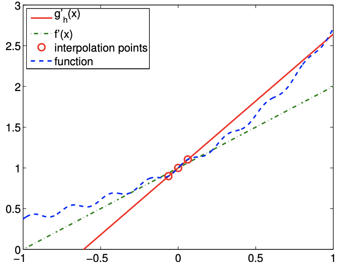
Evaluating the interpolant at \(x=\tilde{x}_{i}\), we obtain \[\begin{aligned} f_{h}^{\prime}\left(\tilde{x}_{i}\right) &=(\mathcal{I} f)^{\prime}\left(\tilde{x}_{i}\right)=\frac{1}{2 \tilde{h}^{2}} f\left(\tilde{x}_{i-1}\right)\left(\tilde{x}_{i}-\tilde{x}_{i+1}\right)+\frac{1}{2 \tilde{h}^{2}} f\left(\tilde{x}_{i+1}\right)\left(\tilde{x}_{i}-\tilde{x}_{i-1}\right) \\ &=\frac{1}{2 \tilde{h}^{2}} f\left(\tilde{x}_{i-1}\right)(-\tilde{h})+\frac{1}{2 \tilde{h}^{2}} f\left(\tilde{x}_{i+1}\right)(\tilde{h}) \\ &=\frac{1}{2 \tilde{h}}\left(f\left(\tilde{x}_{i+1}\right)-f\left(\tilde{x}_{i-1}\right)\right) . \end{aligned}\] Note that even though the quadratic interpolant is constructed from the three interpolation points, only two of the three points are used in estimating the derivative. The approximation procedure is illustrated in Figure 3.4(a).

The error bound for the centered difference is given by \[e_{i}=\left|f\left(\tilde{x}_{i}\right)-f_{h}^{\prime}\left(\tilde{x}_{i}\right)\right| \leq \frac{\tilde{h}^{2}}{6} \max _{x \in\left[\tilde{x}_{i-1}, \tilde{x}_{i+1}\right]}\left|f^{\prime \prime \prime}(x)\right|\] The centered difference formula is second-order accurate, as confirmed by the convergence plot in Figure 3.4(b). Proof. The proof of the error bound follows from Taylor expansion. Recall, assuming \(f^{\prime \prime \prime}(x)\) is bounded in \(\left[\tilde{x}_{i-1}, \tilde{x}_{i+1}\right]\), \[\begin{aligned} &f\left(\tilde{x}_{i+1}\right)=f\left(\tilde{x}_{i}+\tilde{h}\right)=f\left(\tilde{x}_{i}\right)+f^{\prime}\left(\tilde{x}_{i}\right) \tilde{h}+\frac{1}{2} f^{\prime \prime}\left(\tilde{x}_{i}\right) \tilde{h}^{2}+\frac{1}{6} f^{\prime \prime \prime}\left(\xi^{+}\right) \tilde{h}^{3}, \\ &f\left(\tilde{x}_{i-1}\right)=f\left(\tilde{x}_{i}-\tilde{h}\right)=f\left(\tilde{x}_{i}\right)-f^{\prime}\left(\tilde{x}_{i}\right) \tilde{h}+\frac{1}{2} f^{\prime \prime}\left(\tilde{x}_{i}\right) \tilde{h}^{2}-\frac{1}{6} f^{\prime \prime \prime}\left(\xi^{-}\right) \tilde{h}^{3}, \end{aligned}\] for some \(\xi^{+} \in\left[\tilde{x}_{i}, \tilde{x}_{i+1}\right]\) and \(\xi^{-} \in\left[\tilde{x}_{i-1}, \tilde{x}_{i}\right]\). The centered difference formula gives \[\begin{aligned} (\mathcal{I} f)^{\prime}\left(\tilde{x}_{i}\right)=& \frac{1}{2 \tilde{h}}\left(f\left(x_{i+1}\right)-f\left(\tilde{x}_{i-1}\right)\right) \\ =\frac{1}{2 \tilde{h}}\left[\left(f\left(\tilde{x}_{i}\right)+f^{\prime}\left(\tilde{x}_{i}\right) \tilde{h}+\frac{1}{2} f^{\prime \prime}\left(\tilde{x}_{i}\right) \tilde{h}^{2}+\frac{1}{6} f^{\prime \prime \prime}\left(\xi^{+}\right) \tilde{h}^{3}\right)\right.\\ &\left.-\left(f\left(\tilde{x}_{i}\right)-f^{\prime}\left(\tilde{x}_{i}\right) \tilde{h}+\frac{1}{2} f^{\prime \prime}\left(\tilde{x}_{i}\right) \tilde{h}^{2}-\frac{1}{6} f^{\prime \prime \prime}\left(\xi^{-}\right) \tilde{h}^{3}\right)\right] \\ =& f^{\prime}\left(\tilde{x}_{i}\right)+\frac{1}{12} \tilde{h}^{2}\left(f^{\prime \prime \prime}\left(\xi^{+}\right)-f^{\prime \prime \prime}\left(\xi^{-}\right)\right) . \end{aligned}\] The error in the derivative estimate is \[\left|f^{\prime}\left(\tilde{x}_{i}\right)-(\mathcal{I} f)^{\prime}\left(\tilde{x}_{i}\right)\right|=\left|\frac{1}{12} \tilde{h}^{2}\left(f^{\prime \prime \prime}\left(\xi^{+}\right)-f^{\prime \prime \prime}\left(\xi^{-}\right)\right)\right|=\frac{1}{6} \tilde{h}^{2} \max _{x \in\left[\tilde{x}_{i-1}, \tilde{x}_{i+1}\right]}\left|f^{\prime \prime \prime}(x)\right| .\] Using a higher-order interpolation scheme, we can develop higher-order accurate numerical differentiation rules. However, the numerical stencil extends with the approximation order, because the number of interpolation points increases with the interpolation order.

We would also like to make some remarks about how noise affects the quality of numerical differentiation. Let us consider approximating a derivative of \(f(x)=\exp (x)\) at \(x=0\). However, assume that we do not have access to \(f\) itself, but rather a function \(f\) with some small noise added to it. In particular, let us consider \[g(x)=f(x)+\epsilon \sin (k x),\] with \(\epsilon=0.04\) and \(k=1 / \epsilon\). We can think of \(\epsilon \sin (k x)\) as noise added, for example, in a measuring process. Considering \(f(0)=1\), this is a relatively small noise in terms of amplitude.

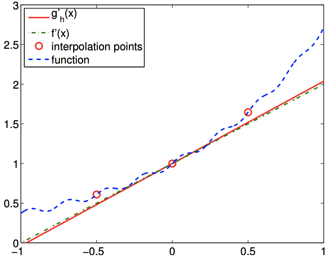
The result of applying the finite difference formulas to \(g\) in an attempt to approximate \(f^{\prime}(0)\) is shown in Figure 3.5. Comparing the approximations obtained for \(\tilde{h}=1 / 2\) and \(1 / 16\), we see that the approximation in fact gets worse as \(\tilde{h}\) is refined. Figure \(3.6\) confirms that all numerical differentiation formulas considered in this section fail to converge. In fact, they all asymptotically commit \(\mathcal{O}(1)\) error as \(\tilde{h} \rightarrow 0\), even though the error decreases to less than \(10^{-2}\) for a certain choice of \(\tilde{h}\).

(a) \(\tilde{h}=1 / 2\)

(b) \(\tilde{h}=1 / 16\)

Figure 3.5: The centered difference formula applied to a noisy function.

Figure 3.6: Convergence of the numerical differentiation formula applied to a noisy function.

As essentially any data taken in real life is inherently noisy, we must be careful when differentiating the data. For example, let us say that our objective is to estimate the acceleration of an object by differentiating a velocity measurement. Due to the presence of measurement noise, we in general cannot expect the quality of our acceleration estimate to improve as we improve the sampling rate and decreasing the discretization scale, \(\tilde{h}\).

One strategy to effectively differentiate a noisy data is to first filter the noisy data. Filtering is a technique to clean a signal by removing frequency content above a certain frequency \({ }_{-}^{3}\) For example, if a user is only interested in estimating the behavior of a signal below a certain frequency, all content above that threshold can be deemed noise. The cleaned data is essentially smooth with respect to the scale of interest, and thus can be safely differentiated. Another alternative, discussed in Unit III, is to first fit a smooth function to many data points and then differentiate this smooth fit.

Second Derivatives

Following the same interpolation-based template, we can develop a numerical approximation to higher-order derivatives. In general, to estimate the \(p^{\text {th }}\)-derivative, we must use an interpolation rule based on \(p^{\text {th }}\) - or higher-degree polynomial reconstruction. As an example, we demonstrate how to estimate the second derivative from a quadratic interpolation.

Example 3.1.4 second-order centered difference

We can use the quadratic interpolant considered in the previous case to estimate the second derivative of the function. Again, choosing \(\bar{x}^{1}=\tilde{x}_{i-1}, \bar{x}^{2}=\tilde{x}_{i}, \bar{x}^{3}=\tilde{x}_{i+1}\) as the interpolation points, the quadratic reconstruction is given by \[(\mathcal{I} f)(x)=f\left(\tilde{x}_{i-1}\right) \phi_{1}(x)+f\left(\tilde{x}_{i}\right) \phi_{2}(x)+f\left(\tilde{x}_{i+1}\right) \phi_{3}(x),\] where the Lagrange basis function are given by \[\begin{gathered} \phi_{1}(x)=\frac{\left(x-\tilde{x}_{i}\right)\left(x-\tilde{x}_{i+1}\right)}{\left(\tilde{x}_{i-1}-\tilde{x}_{i}\right)\left(\tilde{x}_{i-1}-\tilde{x}_{i+1}\right)}, \\ \phi_{2}(x)=\frac{\left(x-\tilde{x}_{i-1}\right)\left(x-\tilde{x}_{i+1}\right)}{\left(\tilde{x}_{i}-\tilde{x}_{i-1}\right)\left(\tilde{x}_{i}-\tilde{x}_{i+1}\right)}, \\ \phi_{3}(x)=\frac{\left(x-\tilde{x}_{i-1}\right)\left(x-\tilde{x}_{i}\right)}{\left(\tilde{x}_{i+1}-\tilde{x}_{i-1}\right)\left(\tilde{x}_{i+1}-\tilde{x}_{i}\right)} . \end{gathered}\] Computing the second derivative of the quadratic interpolant can be proceeded as \[(\mathcal{I} f)^{\prime \prime}(x)=f\left(\tilde{x}_{i-1}\right) \phi_{1}^{\prime \prime}(x)+f\left(\tilde{x}_{i}\right) \phi_{2}^{\prime \prime}(x)+f\left(\tilde{x}_{i+1}\right) \phi_{3}^{\prime \prime}(x) .\] In particular, note that once the second derivatives of the Lagrange basis are evaluated, we can express the second derivative of the interpolant as a sum of the functions evaluated at three points.

\({ }^{3}\) Sometimes signals below a certain frequency is filtered to eliminate the bias. The derivatives of the Lagrange basis are given by \[\begin{gathered} \phi_{1}^{\prime \prime}(x)=\frac{2}{\left(\tilde{x}_{i-1}-\tilde{x}_{i}\right)\left(\tilde{x}_{i-1}-\tilde{x}_{i+1}\right)}=\frac{2}{(-\tilde{h})(-2 \tilde{h})}=\frac{1}{\tilde{h}^{2}}, \\ \phi_{2}^{\prime \prime}(x)=\frac{2}{\left(\tilde{x}_{i}-\tilde{x}_{i-1}\right)\left(\tilde{x}_{i}-\tilde{x}_{i+1}\right)}=\frac{2}{(\tilde{h})(-\tilde{h})}=-\frac{2}{\tilde{h}^{2}}, \\ \phi_{3}^{\prime \prime}(x)=\frac{2}{\left(\tilde{x}_{i+1}-\tilde{x}_{i-1}\right)\left(\tilde{x}_{i+1}-\tilde{x}_{i}\right)}=\frac{2}{(2 \tilde{h})(\tilde{h})}=\frac{1}{\tilde{h}^{2}} . \end{gathered}\] Substitution of the derivatives to the second derivative of the quadratic interpolant yields \[\begin{aligned} (\mathcal{I} f)^{\prime \prime}\left(\tilde{x}_{i}\right) &=f\left(\tilde{x}_{i-1}\right)\left(\frac{1}{\tilde{h}^{2}}\right)+f\left(\tilde{x}_{i}\right)\left(\frac{-2}{\tilde{h}^{2}}\right)+f\left(\tilde{x}_{i+1}\right)\left(\frac{1}{\tilde{h}^{2}}\right) \\ &=\frac{1}{\tilde{h}^{2}}\left(f\left(\tilde{x}_{i-1}\right)-2 f\left(\tilde{x}_{i}\right)+f\left(\tilde{x}_{i+1}\right)\right) . \end{aligned}\] The error in the second-derivative approximation is bounded by \[e_{i} \equiv\left|f^{\prime \prime}\left(\tilde{x}_{i}\right)-(\mathcal{I} f)^{\prime \prime}\left(\tilde{x}_{i}\right)\right| \leq \frac{\tilde{h}^{2}}{12} \max _{x \in\left[\tilde{x}_{i-1}, \tilde{x}_{i+1}\right]}\left|f^{(4)}(x)\right| .\] Thus, the scheme is second-order accurate.

Proof

Let us demonstrate that the second-order derivative formula works for constant, linear, and quadratic function. First, we consider \(f(x)=c\). Clearly, the second derivative is \(f^{\prime \prime}(x)=0\). Using the approximation formula, we obtain \[(\mathcal{I} f)^{\prime \prime}\left(\tilde{x}_{i}\right)=\frac{1}{\tilde{h}^{2}}\left(f\left(\tilde{x}_{i-1}\right)-2 f\left(\tilde{x}_{i}\right)+f\left(\tilde{x}_{i+1}\right)\right)=\frac{1}{\tilde{h}^{2}}(c-2 c+c)=0 .\]

Thus, the approximation provides the exact second derivative for the constant function. This is not surprising, as the error is bounded by the fourth derivative of \(f\), and the fourth derivative of the constant function is zero.

Second, we consider \(f(x)=b x+c\). The second derivative is again \(f^{\prime \prime}(x)=0\). The approximation formula gives \[\begin{aligned} (\mathcal{I} f)^{\prime \prime}\left(\tilde{x}_{i}\right) &=\frac{1}{\tilde{h}^{2}}\left(f\left(\tilde{x}_{i-1}\right)-2 f\left(\tilde{x}_{i}\right)+f\left(\tilde{x}_{i+1}\right)\right)=\frac{1}{\tilde{h}^{2}}\left[\left(b \tilde{x}_{i-1}+c\right)-2\left(b \tilde{x}_{i}+c\right)+\left(b \tilde{x}_{i+1}+c\right)\right] \\ &=\frac{1}{\tilde{h}^{2}}\left[\left(b\left(\tilde{x}_{i}-\tilde{h}\right)+c\right)-2\left(b \tilde{x}_{i}+c\right)+\left(b\left(\tilde{x}_{i}+\tilde{h}\right)+c\right)\right]=0 . \end{aligned}\] Thus, the approximation also works correctly for a linear function.

Finally, let us consider \(f(x)=a x^{2}+b x+c\). The second derivative for this case is \(f^{\prime \prime}(x)=2 a\). The approximation formula gives \[\begin{aligned} (\mathcal{I} f)^{\prime \prime}\left(\tilde{x}_{i}\right) &=\frac{1}{\tilde{h}^{2}}\left[\left(a \tilde{x}_{i-1}^{2}+b \tilde{x}_{i-1}+c\right)-2\left(a \tilde{x}_{i}^{2}+b \tilde{x}_{i}+c\right)+\left(a \tilde{x}_{i+1}^{2}+b \tilde{x}_{i+1}+c\right)\right] \\ &=\frac{1}{\tilde{h}^{2}}\left[\left(a\left(\tilde{x}_{i}-\tilde{h}\right)^{2}+b\left(\tilde{x}_{i}-\tilde{h}\right)+c\right)-2\left(a \tilde{x}_{i}^{2}+b \tilde{x}_{i}+c\right)+\left(a\left(\tilde{x}_{i}+\tilde{h}\right)^{2}+b\left(\tilde{x}_{i}+\tilde{h}\right)+c\right)\right] \\ &=\frac{1}{\tilde{h}^{2}}\left[a\left(\tilde{x}_{i}^{2}-2 \tilde{h} \tilde{x}_{i}+\tilde{h}^{2}\right)-2 a \tilde{x}_{i}^{2}+a\left(\tilde{x}_{i}^{2}+2 \tilde{h} \tilde{x}_{i}+\tilde{h}^{2}\right)\right] \\ &=\frac{1}{\tilde{h}^{2}}\left[2 a \tilde{h}^{2}\right]=2 a \end{aligned}\] Thus, the formula also yields the exact derivative for the quadratic function.

The numerical differentiation rules covered in this section form the basis for the finite difference method - a framework for numerically approximating the solution to differential equations. In the framework, the infinite-dimensional solution on a domain is approximated by a finite number of nodal values on a discretization of the domain. This allows us to approximate the solution to complex differential equations - particularly partial differential equations - that do not have closed form solutions. We will study in detail these numerical methods for differential equations in Unit IV, and we will revisit the differential rules covered in this section at the time.

We briefly note another application of our finite difference formulas: they may be used (say) to approximately evaluate our (say) interpolation error bounds to provide an a posteriori estimate for the error.