4.1: Computer Architecture and Computer Programming

Virtual Processor

It is convenient when programming a computer to have a mental model of the underlying architecture: the components or “units,” functions, and interconnections which ultimately implement the program. It is not important that the mental model directly correspond to the actual hardware of any real computer. But it is important that the mental model lead to the right decisions as regards how to write correct and efficient programs.

We show in Figure 4.1 the architecture for a “virtual computer.” There are many ways in which we can extend or refine our model to more accurately represent either particular processes or particular computers of interest: we might break down each unit into smaller units — for example, a memory hierarchy; we might consider additional, special-purpose, units — for example for graphics and visualization; and we might replicate our virtual computer many times to represent (a system of) many interacting processes. We emphasize that if you put a screwdriver to computer case, you would not find a one-to-one mapping from our virtual entities to corresponding hardware elements. But you might come close.

We now describe the different elements. On the far left we indicate the memory. This memory is often hierarchical: faster and more expensive memory in a “cache”; slower and much more extensive “RAM.” (Note also there will be archival memory outside the processor accessed through I/O functions, as described shortly.) Next there is the arithmetic unit which performs the various “basic” operations on data — for example, assignment, addition, multiplication, and comparison. (The adjective “arithmetic” for this unit is overly restrictive, but since in this course we are primarily focused on numerical methods the key operations are indeed arithmetic.) We also identify the “instruction stack” which contains the instructions necessary to implement the desired program. And finally there is the I/O (Input/Output) unit which controls communication between our processor and external devices and other processes; the latter may take the form of files on archival media (such as disks), keyboards and other user input devices, sensors and actuators (say, on a robot), and displays.

We note that all the components — memory, arithmetic unit, instruction stack, I/O unit are interconnected through buses which shuttle the necessary data between the different elements. The arithmetic unit may receive instructions from the instruction stack and read and write data from memory; similarly, the instruction stack may ask the I/O unit to read data from a file to the memory unit or say write data from memory to a display. And the arithmetic unit may effectively communicate directly with the instruction stack to control the flow of the program. These data buses are of course a model for wires (or optical communication paths) in an actual hardware computer.

Figure 4.1: Virtual Processor

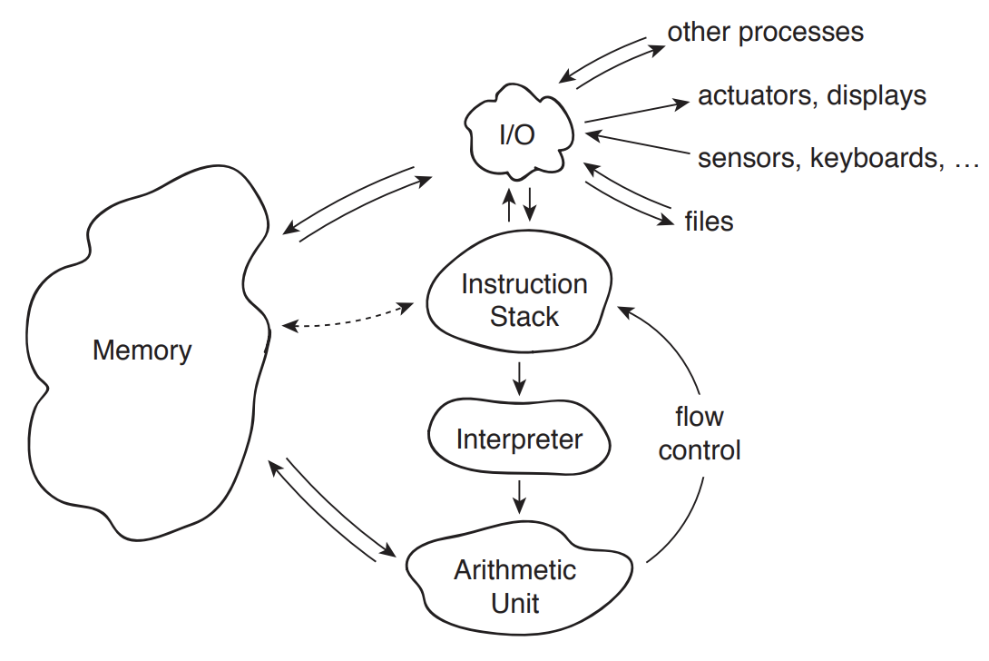
The “I” in Figure 4.1 stands for interpreter. The Interpreter takes a line or lines of a program written in a high-level programming or “scripting” language — such as Matlab or Python — from the instruction stack, translates these instructions into machine code, and then passes these now machine-actionable directives to the arithmetic unit for execution. (Some languages, such as C, are not interpreted but rather compiled: the program is translated en masse into machine code prior to execution. As you might imagine, compiled codes will typically execute faster than interpreted codes.)

There are typically two ways in which an interpreter can feed the arithmetic unit. The first way, more interactive with the user, is “command-line” mode: here a user enters each line, or small batch of lines, from the keyboard to the I/O unit; the I/O unit in turn passes these lines to the interpreter for processing. The second way, much more convenient for anything but the simplest of tasks, is “script” mode: the I/O unit transfers the entire program from a file prepared by the user to the instruction stack; the program is then executed proceeding from the first line to the last. (The latter is in fact a simplification, as we shall see when we discuss flow control and functions.) Script mode permits much faster execution, since the user is out of the loop; script mode also permits much faster development/adaptation, since the user can re-use the same script many times — only changing data, or perhaps making incremental corrections/improvements or modifications.

Matlab Environment

In Matlab the user interface is the command window. The command window provides the prompt >> to let the user know that Matlab is ready to accept inputs. The user can either directly enter lines of Matlab code after the >> prompt in command-line mode; alternatively, in script mode, the user can enter >> myscript.m to execute the entire program myscript.m. The suffix .m indicates that the file contains a Matlab program; files with the .m suffix are affectionately known as “m files.” (We will later encounter Matlab data files, which take the .mat suffix.) Note that most easily we run Matlab programs and subprograms (such as functions, discussed shortly) from the folder which contains these programs; however we can also set “paths” which Matlab will search to find (say) myscript.m.

Matlab in fact provides an entire environment of which the command window is just one (albeit the most important) part. In addition to the command window, there is a “current folder” window which displays the contents of the current directory — typically .m files and .mat files, but perhaps also other “non-Matlab ” (say, document) files — and provides tools for navigation within the file system of the computer. The Matlab environment also includes an editor — invoked by the “Edit” pull-down menu — which permits the user to create and modify .m files. Matlab also provides several forms of “manual”: doc invokes an extensive documentation facility window and search capability; and, even more useful, within the command window >>help keyword will bring up a short description of keyword (which typically but not always will be a Matlab “built–in” function). Similar environments, more or less graphical, exist for other (interpreted) programming languages such as Python.

We note that in actual practice we execute programs within programs within programs. We boot the system to start the Operating System program; we launch Matlab from within in Operating System to enter the Matlab environment; and then within the Matlab environment we run a script to execute our particular (numerical) program. It is the latter on which we have focused in our description above, though the other layers of the hierarchy are much better known to the “general computer user.” It is of course a major and complicated task to orchestrate these different programs at different levels both as regards process control and also memory and file management. We will illustrate how this is done at a much smaller scale when we discuss functions within the particular Matlab context.