15: Motivation

In odometry-based mobile robot navigation, the accuracy of the robot’s dead reckoning pose tracking depends on minimizing slippage between the robot’s wheels and the ground. Even a momentary slip can lead to an error in heading that will cause the error in the robot’s location estimate to grow linearly over its journey. It is thus important to determine the friction coefficient between the robot’s wheels and the ground, which directly affects the robot’s resistance to slippage. Just as importantly, this friction coefficient will significantly affect the performance of the robot: the ability to push loads.

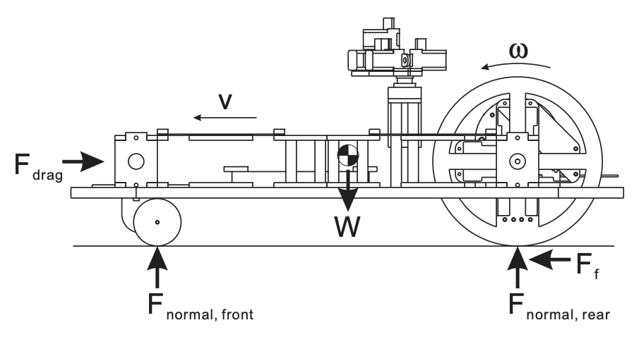
When the mobile robot of Figure \(15.1\) is commanded to move forward, a number of forces come into play. Internally, the drive motors exert a torque (not shown in the figure) on the wheels, which is resisted by the friction force \(F_{\mathrm{f}}\) between the wheels and the ground. If the magnitude of \(F_{\mathrm{f}}\) dictated by the sum of the drag force \(F_{\text {drag }}\) (a combination of all forces resisting the robot’s motion) and the product of the robot’s mass and acceleration is less than the maximum static friction force \(F_{\mathrm{f}, \text { static }}^{\max }\) between the wheels and the ground, the wheels will roll without slipping and the robot will move forward with velocity \(v=\omega r_{\text {wheel }}\). If, however, the magnitude of \(F_{\mathrm{f}}\) reaches \(F_{\mathrm{f} \text {, static }}^{\max }\), the wheels will begin to slip and \(F_{\mathrm{f}}\) will drop to a lower level \(F_{\mathrm{f} \text {, kinetic }}\), the kinetic friction force. The wheels will continue to slip \(\left(v<\omega r_{\text {wheel }}\right.\) ) until zero relative motion between the wheels and the ground is restored (when \(v=\omega r_{\text {wheel }}\) ).

The critical value defining the boundary between rolling and slipping, therefore, is the maximum static friction force. We expect that \[F_{\mathrm{f}, \text { static }}^{\max }=\mu_{\mathrm{s}} F_{\text {normal, rear }},\] where \(\mu_{\mathrm{s}}\) is the static coefficient of friction and \(F_{\text {normal, rear }}\) is the normal force from the ground on the rear, driving, wheels. In order to minimize the risk of slippage (and to be able to push large loads), robot wheels should be designed for a high value of \(\mu_{\mathrm{s}}\) between the wheels and the ground. This value, although difficult to predict accurately by modeling, can be determined by experiment.

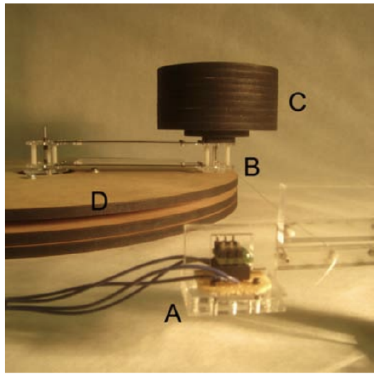
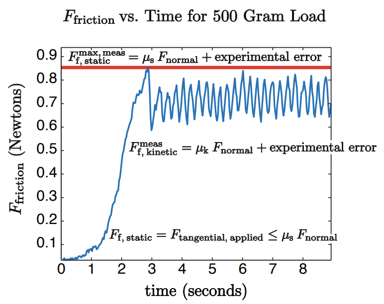
We first conduct experiments for the friction force \(F_{\mathrm{f}, \text { static }}^{\max }\) (in Newtons) as a function of normal load \(F_{\text{normal, applied}}\) (in Newtons) and (nominal) surface area of contact \(A_{\text{surface}}\) (in cm2 ) with the friction turntable apparatus depicted in Figure 15.2. Weights permit us to vary the normal load and "washer" inserts permit us to vary the nominal surface area of contact. A typical experiment (at a particular prescribed value of \(F_{\text {normal, applied }}\) and \(A_{\text {surface }}\) ) yields the time trace of Figure \(15.3\) from which the \(F_{\mathrm{f}, \text { static }}^{\max , \text { means }}\) (our measurement of \(F_{\mathrm{f}, \text { static }}^{\max }\) ) is deduced as the maximum of the response.

We next postulate a dependence (or "model") \[F_{\mathrm{f}, \text { static }}^{\max }\left(F_{\text {normal, applied }}, A_{\text {surface }}\right)=\beta_{0}+\beta_{1} F_{\text {normal, applied }}+\beta_{2} A_{\text {surface }},\] where we expect - but do not a priori assume - from Messieurs Amontons and Coulomb that \(\beta_{0}=0\) and \(\beta_{2}=0\) (and of course \(\beta_{1} \equiv \mu_{\mathrm{s}}\) ). In order to confirm that \(\beta_{0}=0\) and \(\beta_{2}=0\) - or at least confirm that \(\beta_{0}=0\) and \(\beta_{2}=0\) is not untrue - and to find a good estimate for \(\beta_{1} \equiv \mu_{\mathrm{s}}\), we must appeal to our measurements.

The mathematical techniques by which to determine \(\mu_{\mathrm{s}}\) (and \(\beta_{0}, \beta_{2}\) ) "with some confidence" from noisy experimental data is known as regression, which is the subject of Chapter 19. Regression, in turn, is best described in the language of linear algebra (Chapter 16), and is built upon the linear algebra concept of least squares (Chapter 17).