16.1: Basic Vector and Matrix Operations

Definitions

Let us first introduce the primitive objects in linear algebra: vectors and matrices. A \(m\)-vector \(v \in \mathbb{R}^{m \times 1}\) consists of \(m\) real numbers \(\stackrel{1}{-}\) \[v=\left(\begin{array}{c} v_{1} \\ v_{2} \\ \vdots \\ v_{m} \end{array}\right) .\] It is also called a column vector, which is the default vector in linear algebra. Thus, by convention, \(v \in \mathbb{R}^{m}\) implies that \(v\) is a column vector in \(\mathbb{R}^{m \times 1}\). Note that we use subscript \((\cdot)_{i}\) to address the \(i\)-th component of a vector. The other kind of vector is a row vector \(v \in \mathbb{R}^{1 \times n}\) consisting of \(n\) entries \[v=\left(\begin{array}{llll} v_{1} & v_{2} & \cdots & v_{n} \end{array}\right) .\] Let us consider a few examples of column and row vectors.

Example 16.1.1 vectors

Examples of (column) vectors in \(\mathbb{R}^{3}\) are \[v=\left(\begin{array}{l} 1 \\ 3 \\ 6 \end{array}\right), \quad u=\left(\begin{array}{c} \sqrt{3} \\ -7 \\ \pi \end{array}\right), \quad \text { and } \quad w=\left(\begin{array}{c} 9.1 \\ 7 / 3 \\ \sqrt{\pi} \end{array}\right) .\] \({ }^{1}\) The concept of vectors readily extends to complex numbers, but we only consider real vectors in our presentation of this chapter.

To address a specific component of the vectors, we write, for example, \(v_{1}=1, u_{1}=\sqrt{3}\), and \(w_{3}=\sqrt{\pi}\). Examples of row vectors in \(\mathbb{R}^{1 \times 4}\) are \[v=\left(\begin{array}{llll} 2 & -5 & \sqrt{2} & e \end{array}\right) \text { and } u=\left(\begin{array}{llll} -\sqrt{\pi} & 1 & 1 & 0 \end{array}\right) .\] Some of the components of these row vectors are \(v_{2}=-5\) and \(u_{4}=0\).

A matrix \(A \in \mathbb{R}^{m \times n}\) consists of \(m\) rows and \(n\) columns for the total of \(m \cdot n\) entries, \[A=\left(\begin{array}{cccc} A_{11} & A_{12} & \cdots & A_{1 n} \\ A_{21} & A_{22} & \cdots & A_{2 n} \\ \vdots & \vdots & \ddots & \vdots \\ A_{m 1} & A_{m 2} & \cdots & A_{m n} \end{array}\right)\] Extending the convention for addressing an entry of a vector, we use subscript \((\cdot)_{i j}\) to address the entry on the \(i\)-th row and \(j\)-th column. Note that the order in which the row and column are referred follows that for describing the size of the matrix. Thus, \(A \in \mathbb{R}^{m \times n}\) consists of entries \[A_{i j}, \quad i=1, \ldots, m, \quad j=1, \ldots, n .\] Sometimes it is convenient to think of a (column) vector as a special case of a matrix with only one column, i.e., \(n=1\). Similarly, a (row) vector can be thought of as a special case of a matrix with \(m=1\). Conversely, an \(m \times n\) matrix can be viewed as \(m\) row \(n\)-vectors or \(n\) column \(m\)-vectors, as we discuss further below.

Example 16.1.2 matrices

Examples of matrices are \[A=\left(\begin{array}{cc} 1 & \sqrt{3} \\ -4 & 9 \\ \pi & -3 \end{array}\right) \quad \text { and } \quad B=\left(\begin{array}{ccc} 0 & 0 & 1 \\ -2 & 8 & 1 \\ 0 & 3 & 0 \end{array}\right) \text {. }\] The matrix \(A\) is a \(3 \times 2\) matrix \(\left(A \in \mathbb{R}^{3 \times 2}\right)\) and matrix \(B\) is a \(3 \times 3\) matrix \(\left(B \in \mathbb{R}^{3 \times 3}\right)\). We can also address specific entries as, for example, \(A_{12}=\sqrt{3}, A_{31}=-4\), and \(B_{32}=3\).

While vectors and matrices may appear like arrays of numbers, linear algebra defines special set of rules to manipulate these objects. One such operation is the transpose operation considered next.

Transpose Operation

The first linear algebra operator we consider is the transpose operator, denoted by superscript \((\cdot)^{\mathrm{T}}\). The transpose operator swaps the rows and columns of the matrix. That is, if \(B=A^{\mathrm{T}}\) with \(A \in \mathbb{R}^{m \times n}\), then \[B_{i j}=A_{j i}, \quad 1 \leq i \leq n, \quad 1 \leq j \leq m .\] Because the rows and columns of the matrix are swapped, the dimensions of the matrix are also swapped, i.e., if \(A \in \mathbb{R}^{m \times n}\) then \(B \in \mathbb{R}^{n \times m}\).

If we swap the rows and columns twice, then we return to the original matrix. Thus, the transpose of a transposed matrix is the original matrix, i.e. \[\left(A^{\mathrm{T}}\right)^{\mathrm{T}}=A\]

Example 16.1.3 transpose

Let us consider a few examples of transpose operation. A matrix \(A\) and its transpose \(B=A^{\mathrm{T}}\) are related by \[A=\left(\begin{array}{cc} 1 & \sqrt{3} \\ -4 & 9 \\ \pi & -3 \end{array}\right) \quad \text { and } \quad B=\left(\begin{array}{ccc} 1 & -4 & \pi \\ \sqrt{3} & 9 & -3 \end{array}\right)\] The rows and columns are swapped in the sense that \(A_{31}=B_{13}=\pi\) and \(A_{12}=B_{21}=\sqrt{3}\). Also, because \(A \in \mathbb{R}^{3 \times 2}, B \in \mathbb{R}^{2 \times 3}\). Interpreting a vector as a special case of a matrix with one column, we can also apply the transpose operator to a column vector to create a row vector, i.e., given \[v=\left(\begin{array}{c} \sqrt{3} \\ -7 \\ \pi \end{array}\right)\] the transpose operation yields \[u=v^{\mathrm{T}}=\left(\begin{array}{lll} \sqrt{3} & -7 & \pi \end{array}\right) .\] Note that the transpose of a column vector is a row vector, and the transpose of a row vector is a column vector.

Vector Operations

The first vector operation we consider is multiplication of a vector \(v \in \mathbb{R}^{m}\) by a scalar \(\alpha \in \mathbb{R}\). The operation yields \[u=\alpha v,\] where each entry of \(u \in \mathbb{R}^{m}\) is given by \[u_{i}=\alpha v_{i}, \quad i=1, \ldots, m .\] In other words, multiplication of a vector by a scalar results in each component of the vector being scaled by the scalar.

The second operation we consider is addition of two vectors \(v \in \mathbb{R}^{m}\) and \(w \in \mathbb{R}^{m}\). The addition yields \[u=v+w,\] where each entry of \(u \in \mathbb{R}^{m}\) is given by \[u_{i}=v_{i}+w_{i}, \quad i=1, \ldots, m .\] In order for addition of two vectors to make sense, the vectors must have the same number of components. Each entry of the resulting vector is simply the sum of the corresponding entries of the two vectors.

We can summarize the action of the scaling and addition operations in a single operation. Let \(v \in \mathbb{R}^{m}, w \in \mathbb{R}^{m}\) and \(\alpha \in \mathbb{R}\). Then, the operation \[u=v+\alpha w\]

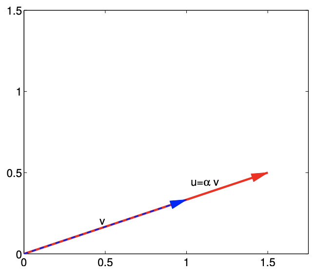
(a) scalar scaling

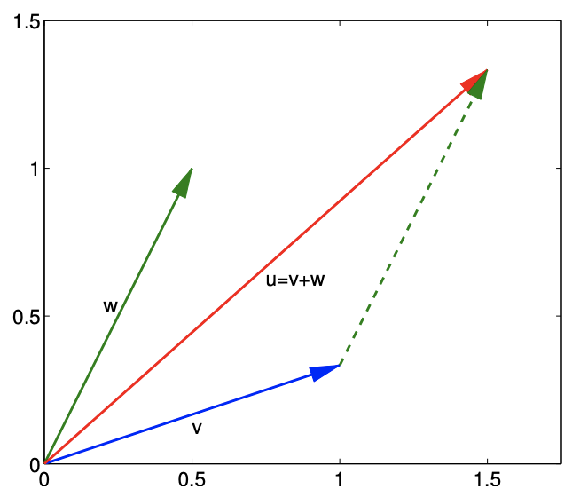
(b) vector addition

Figure 16.1: Illustration of vector scaling and vector addition.

yields a vector \(u \in \mathbb{R}^{m}\) whose entries are given by \[u_{i}=v_{i}+\alpha w_{i}, \quad i=1, \ldots, m .\] The result is nothing more than a combination of the scalar multiplication and vector addition rules.

Example 16.1.4 vector scaling and addition in \(\mathbb{R}^{2}\)

Let us illustrate scaling of a vector by a scalar and addition of two vectors in \(\mathbb{R}^{2}\) using \[v=\left(\begin{array}{c} 1 \\ 1 / 3 \end{array}\right) \quad, w=\left(\begin{array}{c} 1 / 2 \\ 1 \end{array}\right), \quad \text { and } \quad \alpha=\frac{3}{2} .\] First, let us consider scaling of the vector \(v\) by the scalar \(\alpha\). The operation yields \[u=\alpha v=\frac{3}{2}\left(\begin{array}{c} 1 \\ 1 / 3 \end{array}\right)=\left(\begin{array}{c} 3 / 2 \\ 1 / 2 \end{array}\right) .\] This operation is illustrated in Figure 16.1(a). The vector \(v\) is simply stretched by the factor of \(3 / 2\) while preserving the direction.

Now, let us consider addition of the vectors \(v\) and \(w\). The vector addition yields \[u=v+w=\left(\begin{array}{c} 1 \\ 1 / 3 \end{array}\right)+\left(\begin{array}{c} 1 / 2 \\ 1 \end{array}\right)=\left(\begin{array}{c} 3 / 2 \\ 4 / 3 \end{array}\right) .\] Figure \(16.1(b)\) illustrates the vector addition process. We translate \(w\) so that it starts from the tip of \(v\) to form a parallelogram. The resultant vector is precisely the sum of the two vectors. Note that the geometric intuition for scaling and addition provided for \(\mathbb{R}^{2}\) readily extends to higher dimensions.

Example 16.1.5 vector scaling and addition in \(\mathbb{R}^{3}\)

Let \(v=\left(\begin{array}{lll}1 & 3 & 6\end{array}\right)^{\mathrm{T}}, w=\left(\begin{array}{ccc}2 & -1 & 0\end{array}\right)^{\mathrm{T}}\), and \(\alpha=3\). Then, \[u=v+\alpha w=\left(\begin{array}{l} 1 \\ 3 \\ 6 \end{array}\right)+3 \cdot\left(\begin{array}{c} 2 \\ -1 \\ 0 \end{array}\right)=\left(\begin{array}{l} 1 \\ 3 \\ 6 \end{array}\right)+\left(\begin{array}{c} 6 \\ -3 \\ 0 \end{array}\right)=\left(\begin{array}{l} 7 \\ 0 \\ 6 \end{array}\right)\]

Inner Product

Another important operation is the inner product. This operation takes two vectors of the same dimension, \(v \in \mathbb{R}^{m}\) and \(w \in \mathbb{R}^{m}\), and yields a scalar \(\beta \in \mathbb{R}\) : \[\beta=v^{\mathrm{T}} w \quad \text { where } \quad \beta=\sum_{i=1}^{m} v_{i} w_{i} .\] The appearance of the transpose operator will become obvious once we introduce the matrix-matrix multiplication rule. The inner product in a Euclidean vector space is also commonly called the dot product and is denoted by \(\beta=v \cdot w\). More generally, the inner product of two elements of a vector space is denoted by \((\cdot, \cdot)\), i.e., \(\beta=(v, w)\).

Example 16.1.6 inner product

Let us consider two vectors in \(\mathbb{R}^{3}, v=\left(\begin{array}{lll}1 & 3 & 6\end{array}\right)^{\mathrm{T}}\) and \(w=\left(\begin{array}{ccc}2 & -1 & 0\end{array}\right)^{\mathrm{T}}\). The inner product of these two vectors is \[\beta=v^{\mathrm{T}} w=\sum_{i=1}^{3} v_{i} w_{i}=1 \cdot 2+3 \cdot(-1)+6 \cdot 0=-1 .\]

(2-Norm)

Using the inner product, we can naturally define the 2 -norm of a vector. Given \(v \in \mathbb{R}^{m}\), the 2 -norm of \(v\), denoted by \(\|v\|_{2}\), is defined by \[\|v\|_{2}=\sqrt{v^{\mathrm{T}} v}=\sqrt{\sum_{i=1}^{m} v_{i}^{2}} .\] Note that the norm of any vector is non-negative, because it is a sum \(m\) non-negative numbers (squared values). The \(\ell_{2}\) norm is the usual Euclidean length; in particular, for \(m=2\), the expression simplifies to the familiar Pythagorean theorem, \(\|v\|_{2}=\sqrt{v_{1}^{2}+v_{2}^{2}}\). While there are other norms, we almost exclusively use the 2 -norm in this unit. Thus, for notational convenience, we will drop the subscript 2 and write the 2 -norm of \(v\) as \(\|v\|\) with the implicit understanding \(\|\cdot\| \equiv\|\cdot\|_{2}\).

By definition, any norm must satisfy the triangle inequality, \[\|v+w\| \leq\|v\|+\|w\|,\] for any \(v, w \in \mathbb{R}^{m}\). The theorem states that the sum of the lengths of two adjoining segments is longer than the distance between their non-joined end points, as is intuitively clear from Figure \(16.1\) (b). For norms defined by inner products, as our 2-norm above, the triangle inequality is automatically satisfied.

Proof

For norms induced by an inner product, the proof of the triangle inequality follows directly from the definition of the norm and the Cauchy-Schwarz inequality. First, we expand the expression as \[\|v+w\|^{2}=(v+w)^{\mathrm{T}}(v+w)=v^{\mathrm{T}} v+2 v^{\mathrm{T}} w+w^{\mathrm{T}} w .\] The middle terms can be bounded by the Cauchy-Schwarz inequality, which states that \[v^{\mathrm{T}} w \leq\left|v^{\mathrm{T}} w\right| \leq\|v\|\|w\| .\] Thus, we can bound the norm as \[\|v+w\|^{2} \leq\|v\|^{2}+2\|v\|\|w\|+\|w\|^{2}=(\|v\|+\|w\|)^{2},\] and taking the square root of both sides yields the desired result.

Example 16.1.7 norm of a vector

Let \(v=\left(\begin{array}{ccc}1 & 3 & 6\end{array}\right)^{\mathrm{T}}\) and \(w=\left(\begin{array}{ccc}2 & -1 & 0\end{array}\right)^{\mathrm{T}}\). The \(\ell_{2}\) norms of these vectors are \[\begin{gathered} \|v\|=\sqrt{\sum_{i=1}^{3} v_{i}^{2}}=\sqrt{1^{2}+3^{2}+6^{2}}=\sqrt{46} \\ \text { and } \quad\|w\|=\sqrt{\sum_{i=1}^{3} w_{i}^{2}}=\sqrt{2^{2}+(-1)^{2}+0^{2}}=\sqrt{5} . \end{gathered}\]

Example 16.1.8 triangle inequality

Let us illustrate the triangle inequality using two vectors \[v=\left(\begin{array}{c} 1 \\ 1 / 3 \end{array}\right) \quad \text { and } \quad w=\left(\begin{array}{c} 1 / 2 \\ 1 \end{array}\right) .\] The length (or the norm) of the vectors are \[\|v\|=\sqrt{\frac{10}{9}} \approx 1.054 \text { and }\|w\|=\sqrt{\frac{5}{4}} \approx 1.118 .\] On the other hand, the sum of the two vectors is \[v+w=\left(\begin{array}{c} 1 \\ 1 / 3 \end{array}\right)+\left(\begin{array}{c} 1 / 2 \\ 1 \end{array}\right)=\left(\begin{array}{c} 3 / 2 \\ 4 / 3 \end{array}\right)\]

Figure 16.2: Illustration of the triangle inequality.

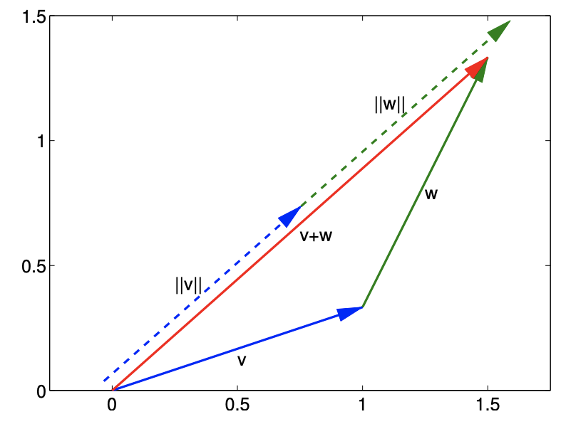
and its length is \[\|v+w\|=\frac{\sqrt{145}}{6} \approx 2.007 .\] The norm of the sum is shorter than the sum of the norms, which is \[\|v\|+\|w\| \approx 2.172 .\] This inequality is illustrated in Figure 16.2. Clearly, the length of \(v+w\) is strictly less than the sum of the lengths of \(v\) and \(w\) (unless \(v\) and \(w\) align with each other, in which case we obtain equality).

In two dimensions, the inner product can be interpreted as \[v^{\mathrm{T}} w=\|v\|\|w\| \cos (\theta),\] where \(\theta\) is the angle between \(v\) and \(w\). In other words, the inner product is a measure of how well \(v\) and \(w\) align with each other. Note that we can show the Cauchy-Schwarz inequality from the above equality. Namely, \(|\cos (\theta)| \leq 1\) implies that \[\left|v^{\mathrm{T}} w\right|=\|v\|\|w\||| \cos (\theta) \mid \leq\|v\|\|w\| .\] In particular, we see that the inequality holds with equality if and only if \(\theta=0\) or \(\pi\), which corresponds to the cases where \(v\) and \(w\) align. It is easy to demonstrate Eq. (16.1) in two dimensions.

Proof

Noting \(v, w \in \mathbb{R}^{2}\), we express them in polar coordinates \[v=\|v\|\left(\begin{array}{c} \cos \left(\theta_{v}\right) \\ \sin \left(\theta_{v}\right) \end{array}\right) \text { and } w=\|w\|\left(\begin{array}{c} \cos \left(\theta_{w}\right) \\ \sin \left(\theta_{w}\right) \end{array}\right) .\] The inner product of the two vectors yield \[\begin{aligned} \beta &=v^{\mathrm{T}} w=\sum_{i=1}^{2} v_{i} w_{i}=\|v\| \cos \left(\theta_{v}\right)\|w\| \cos \left(\theta_{w}\right)+\|v\| \sin \left(\theta_{v}\right)\|w\| \sin \left(\theta_{w}\right) \\ &=\|v\|\|w\|\left(\cos \left(\theta_{v}\right) \cos \left(\theta_{w}\right)+\sin \left(\theta_{v}\right) \sin \left(\theta_{w}\right)\right) \\ &=\|v\|\|w\|\left(\frac{1}{2}\left(e^{i \theta_{v}}+e^{-i \theta_{v}}\right) \frac{1}{2}\left(e^{i \theta_{w}}+e^{-i \theta_{w}}\right)+\frac{1}{2 i}\left(e^{i \theta_{v}}-e^{-i \theta_{v}}\right) \frac{1}{2 i}\left(e^{i \theta_{w}}-e^{-i \theta_{w}}\right)\right) \\ &=\|v\|\|w\|\left(\frac{1}{4}\left(e^{i\left(\theta_{v}+\theta_{w}\right)}+e^{-i\left(\theta_{v}+\theta_{w}\right)}+e^{i\left(\theta_{v}-\theta_{w}\right)}+e^{-i\left(\theta_{v}-\theta_{w}\right)}\right)\right.\\ &\left.\quad-\frac{1}{4}\left(e^{i\left(\theta_{v}+\theta_{w}\right)}+e^{-i\left(\theta_{v}+\theta_{w}\right)}-e^{i\left(\theta_{v}-\theta_{w}\right)}-e^{-i\left(\theta_{v}-\theta_{w}\right)}\right)\right) \\ &=\|v\|\|w\|\left(\frac{1}{2}\left(e^{i\left(\theta_{v}-\theta_{w}\right)}+e^{-i\left(\theta_{v}-\theta_{w}\right)}\right)\right) \\ &=\|v\|\|w\| \cos \left(\theta_{v}-\theta_{w}\right)=\|v\|\|w\| \cos (\theta), \end{aligned}\] where the last equality follows from the definition \(\theta \equiv \theta_{v}-\theta_{w}\).

Begin Advanced Material

For completeness, let us introduce a more general class of norms.

Example 16.1.9 \(p\)-norms

The 2-norm, which we will almost exclusively use, belong to a more general class of norms, called the \(p\)-norms. The \(p\)-norm of a vector \(v \in \mathbb{R}^{m}\) is \[\|v\|_{p}=\left(\sum_{i=1}^{m}\left|v_{i}\right|^{p}\right)^{1 / p}\] where \(p \geq 1\). Any \(p\)-norm satisfies the positivity requirement, the scalar scaling requirement, and the triangle inequality. We see that 2 -norm is a case of \(p\)-norm with \(p=2\).

Another case of \(p\)-norm that we frequently encounter is the 1-norm, which is simply the sum of the absolute value of the entries, i.e. \[\|v\|_{1}=\sum_{i=1}^{m}\left|v_{i}\right| .\] The other one is the infinity norm given by \[\|v\|_{\infty}=\lim _{p \rightarrow \infty}\|v\|_{p}=\max _{i=1, \ldots, m}\left|v_{i}\right| .\] In other words, the infinity norm of a vector is its largest entry in absolute value.

Advanced Material

Figure 16.3: Set of vectors considered to illustrate orthogonality.

Orthogonality

Two vectors \(v \in \mathbb{R}^{m}\) and \(w \in \mathbb{R}^{m}\) are said to be orthogonal to each other if \[v^{\mathrm{T}} w=0\] In two dimensions, it is easy to see that \[v^{\mathrm{T}} w=\|v\|\|w\| \cos (\theta)=0 \Rightarrow \cos (\theta)=0 \Rightarrow \theta=\pi / 2\] That is, the angle between \(v\) and \(w\) is \(\pi / 2\), which is the definition of orthogonality in the usual geometric sense.

Example 16.1.10 orthogonality

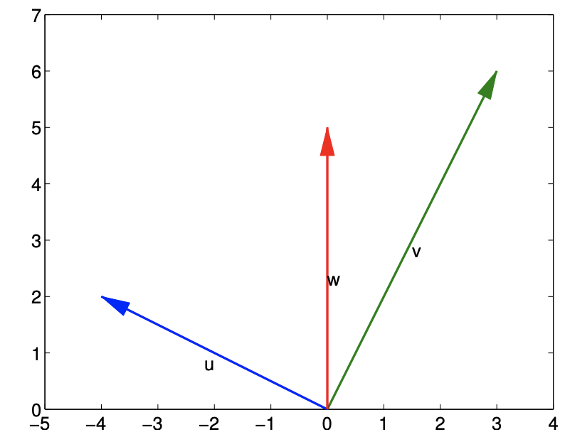
Let us consider three vectors in \(\mathbb{R}^{2}\), \[u=\left(\begin{array}{c} -4 \\ 2 \end{array}\right), \quad v=\left(\begin{array}{c} 3 \\ 6 \end{array}\right), \quad \text { and } \quad w=\left(\begin{array}{c} 0 \\ 5 \end{array}\right)\] and compute three inner products formed by these vectors: \[\begin{gathered} u^{\mathrm{T}} v=-4 \cdot 3+2 \cdot 6=0 \\ u^{\mathrm{T}} w=-4 \cdot 0+2 \cdot 5=10 \\ v^{\mathrm{T}} w=3 \cdot 0+6 \cdot 5=30 \end{gathered}\] Because \(u^{\mathrm{T}} v=0\), the vectors \(u\) and \(v\) are orthogonal to each other. On the other hand, \(u^{\mathrm{T}} w \neq 0\) and the vectors \(u\) and \(w\) are not orthogonal to each other. Similarly, \(v\) and \(w\) are not orthogonal to each other. These vectors are plotted in Figure \(16.3\); the figure confirms that \(u\) and \(v\) are orthogonal in the usual geometric sense.

Figure 16.4: An orthonormal set of vectors

Orthonormality

Two vectors \(v \in \mathbb{R}^{m}\) and \(w \in \mathbb{R}^{m}\) are said to be orthonormal to each other if they are orthogonal to each other and each has unit length, i.e. \[v^{\mathrm{T}} w=0 \quad \text { and } \quad\|v\|=\|w\|=1\]

Example 16.1.11 orthonormality

Two vectors \[u=\frac{1}{\sqrt{5}}\left(\begin{array}{c} -2 \\ 1 \end{array}\right) \quad \text { and } \quad v=\frac{1}{\sqrt{5}}\left(\begin{array}{l} 1 \\ 2 \end{array}\right)\] are orthonormal to each other. It is straightforward to verify that they are orthogonal to each other \[u^{\mathrm{T}} v=\frac{1}{\sqrt{5}}\left(\begin{array}{c} -2 \\ 1 \end{array}\right)^{\mathrm{T}} \frac{1}{\sqrt{5}}\left(\begin{array}{l} 1 \\ 2 \end{array}\right)=\frac{1}{5}\left(\begin{array}{c} -2 \\ 1 \end{array}\right)^{\mathrm{T}}\left(\begin{array}{l} 1 \\ 2 \end{array}\right)=0\] and that each of them have unit length \[\begin{aligned} &\|u\|=\sqrt{\frac{1}{5}\left((-2)^{2}+1^{2}\right)}=1 \\ &\|v\|=\sqrt{\frac{1}{5}\left((1)^{2}+2^{2}\right)}=1 \end{aligned}\] Figure \(16.4\) shows that the vectors are orthogonal and have unit length in the usual geometric sense.

Linear Combinations

Let us consider a set of \(n m\)-vectors \[v^{1} \in \mathbb{R}^{m}, v^{2} \in \mathbb{R}^{m}, \ldots, v^{n} \in \mathbb{R}^{m}\] A linear combination of the vectors is given by \[w=\sum_{j=1}^{n} \alpha^{j} v^{j}\] where \(\alpha^{1}, \alpha^{2}, \ldots, \alpha^{n}\) is a set of real numbers, and each \(v^{j}\) is an \(m\)-vector.

Example 16.1.12 linear combination of vectors

Let us consider three vectors in \(\mathbb{R}^{2}, v^{1}=(-4,2)^{\mathrm{T}}, v^{2}=(36)^{\mathrm{T}}\), and \(v^{3}=(0 \quad 5)\). linear combination of the vectors, with \(\alpha^{1}=1, \alpha^{2}=-2\), and \(\alpha^{3}=3\), is \[\begin{aligned} w &=\sum_{j=1}^{3} \alpha^{j} v^{j}=1 \cdot\left(\begin{array}{c} -4 \\ 2 \end{array}\right)+(-2) \cdot\left(\begin{array}{c} 3 \\ 6 \end{array}\right)+3 \cdot\left(\begin{array}{l} 0 \\ 5 \end{array}\right) \\ &=\left(\begin{array}{c} -4 \\ 2 \end{array}\right)+\left(\begin{array}{c} -6 \\ -12 \end{array}\right)+\left(\begin{array}{c} 0 \\ 15 \end{array}\right)=\left(\begin{array}{c} -10 \\ 5 \end{array}\right) \end{aligned}\] Another example of linear combination, with \(\alpha^{1}=1, \alpha^{2}=0\), and \(\alpha^{3}=0\), is \[w=\sum_{j=1}^{3} \alpha^{j} v^{j}=1 \cdot\left(\begin{array}{c} -4 \\ 2 \end{array}\right)+0 \cdot\left(\begin{array}{l} 3 \\ 6 \end{array}\right)+0 \cdot\left(\begin{array}{c} 0 \\ 5 \end{array}\right)=\left(\begin{array}{c} -4 \\ 2 \end{array}\right)\] Note that a linear combination of a set of vectors is simply a weighted sum of the vectors.

Linear Independence

A set of \(n m\)-vectors are linearly independent if \[\sum_{j=1}^{n} \alpha^{j} v^{j}=0 \quad \text { only if } \quad \alpha^{1}=\alpha^{2}=\cdots=\alpha^{n}=0\] Otherwise, the vectors are linearly dependent.

Example 16.1.13 linear independence

Let us consider four vectors, \[w^{1}=\left(\begin{array}{l} 2 \\ 0 \\ 0 \end{array}\right), \quad w^{2}=\left(\begin{array}{l} 0 \\ 0 \\ 3 \end{array}\right), \quad w^{3}=\left(\begin{array}{c} 0 \\ 1 \\ 0 \end{array}\right), \quad \text { and } \quad w^{4}=\left(\begin{array}{l} 2 \\ 0 \\ 5 \end{array}\right)\] The set of vectors \(\left\{w^{1}, w^{2}, w^{4}\right\}\) is linearly dependent because \[1 \cdot w^{1}+\frac{5}{3} \cdot w^{2}-1 \cdot w^{4}=1 \cdot\left(\begin{array}{l} 2 \\ 0 \\ 0 \end{array}\right)+\frac{5}{3} \cdot\left(\begin{array}{l} 0 \\ 0 \\ 3 \end{array}\right)-1 \cdot\left(\begin{array}{l} 2 \\ 0 \\ 5 \end{array}\right)=\left(\begin{array}{l} 0 \\ 0 \\ 0 \end{array}\right)\] the linear combination with the weights \(\{1,5 / 3,-1\}\) produces the zero vector. Note that the choice of the weights that achieves this is not unique; we just need to find one set of weights to show that the vectors are not linearly independent (i.e., are linearly dependent).

On the other hand, the set of vectors \(\left\{w^{1}, w^{2}, w^{3}\right\}\) is linearly independent. Considering a linear combination, \[\alpha^{1} w^{1}+\alpha^{2} w^{2}+\alpha^{3} w^{3}=\alpha^{1} \cdot\left(\begin{array}{l} 2 \\ 0 \\ 0 \end{array}\right)+\alpha^{2} \cdot\left(\begin{array}{l} 0 \\ 0 \\ 3 \end{array}\right)+\alpha^{3} \cdot\left(\begin{array}{l} 0 \\ 1 \\ 0 \end{array}\right)=\left(\begin{array}{l} 0 \\ 0 \\ 0 \end{array}\right)\] we see that we must choose \(\alpha^{1}=0\) to set the first component to \(0, \alpha^{2}=0\) to set the third component to 0 , and \(\alpha^{3}=0\) to set the second component to 0 . Thus, only way to satisfy the equation is to choose the trivial set of weights, \(\{0,0,0\}\). Thus, the set of vectors \(\left\{w^{1}, w^{2}, w^{3}\right\}\) is linearly independent.

Begin Advanced Material

Vector Spaces and Bases

Given a set of \(n m\)-vectors, we can construct a vector space, \(V\), given by \[V=\operatorname{span}\left(\left\{v^{1}, v^{2}, \ldots, v^{n}\right\}\right),\] where \[\begin{aligned} \operatorname{span}\left(\left\{v^{1}, v^{2}, \ldots, v^{n}\right\}\right) &=\left\{v \in \mathbb{R}^{m}: v=\sum_{k=1}^{n} \alpha^{k} v^{k}, \alpha^{k} \in \mathbb{R}^{n}\right\} \\ &=\text { space of vectors which are linear combinations of } v^{1}, v^{2}, \ldots, v^{n} . \end{aligned}\] In general we do not require the vectors \(\left\{v^{1}, \ldots, v^{n}\right\}\) to be linearly independent. When they are linearly independent, they are said to be a basis of the space. In other words, a basis of the vector space \(V\) is a set of linearly independent vectors that spans the space. As we will see shortly in our example, there are many bases for any space. However, the number of vectors in any bases for a given space is unique, and that number is called the dimension of the space. Let us demonstrate the idea in a simple example.

Example 16.1.14 Bases for a vector space in \(\mathbb{R}^{3}\)

Let us consider a vector space \(V\) spanned by vectors \[v^{1}=\left(\begin{array}{l} 1 \\ 2 \\ 0 \end{array}\right) \quad v^{2}=\left(\begin{array}{c} 2 \\ 1 \\ 0 \end{array}\right) \quad \text { and } \quad v^{3}=\left(\begin{array}{l} 0 \\ 1 \\ 0 \end{array}\right) .\] By definition, any vector \(x \in V\) is of the form \[x=\alpha^{1} v^{1}+\alpha^{2} v^{2}+\alpha^{3} v^{3}=\alpha^{1}\left(\begin{array}{l} 1 \\ 2 \\ 0 \end{array}\right)+\alpha^{2}\left(\begin{array}{l} 2 \\ 1 \\ 0 \end{array}\right)+\alpha^{3}\left(\begin{array}{l} 0 \\ 1 \\ 0 \end{array}\right)=\left(\begin{array}{c} \alpha^{1}+2 \alpha^{2} \\ 2 \alpha^{1}+\alpha^{2}+\alpha^{3} \\ 0 \end{array}\right) .\] Clearly, we can express any vector of the form \(x=\left(x_{1}, x_{2}, 0\right)^{\mathrm{T}}\) by choosing the coefficients \(\alpha^{1}\), \(\alpha^{2}\), and \(\alpha^{3}\) judiciously. Thus, our vector space consists of vectors of the form \(\left(x_{1}, x_{2}, 0\right)^{\mathrm{T}}\), i.e., all vectors in \(\mathbb{R}^{3}\) with zero in the third entry.

We also note that the selection of coefficients that achieves \(\left(x_{1}, x_{2}, 0\right)^{\mathrm{T}}\) is not unique, as it requires solution to a system of two linear equations with three unknowns. The non-uniqueness of the coefficients is a direct consequence of \(\left\{v^{1}, v^{2}, v^{3}\right\}\) not being linearly independent. We can easily verify the linear dependence by considering a non-trivial linear combination such as \[2 v^{1}-v^{2}-3 v^{3}=2 \cdot\left(\begin{array}{l} 1 \\ 2 \\ 0 \end{array}\right)-1 \cdot\left(\begin{array}{l} 2 \\ 1 \\ 0 \end{array}\right)-3 \cdot\left(\begin{array}{l} 0 \\ 1 \\ 0 \end{array}\right)=\left(\begin{array}{l} 0 \\ 0 \\ 0 \end{array}\right)\] Because the vectors are not linearly independent, they do not form a basis of the space.

To choose a basis for the space, we first note that vectors in the space \(V\) are of the form \(\left(x_{1}, x_{2}, 0\right)^{\mathrm{T}}\). We observe that, for example, \[w^{1}=\left(\begin{array}{l} 1 \\ 0 \\ 0 \end{array}\right) \quad \text { and } \quad w^{2}=\left(\begin{array}{l} 0 \\ 1 \\ 0 \end{array}\right)\] would span the space because any vector in \(V\) - a vector of the form \(\left(x_{1}, x_{2}, 0\right)^{\mathrm{T}}\) — can be expressed as a linear combination, \[\left(\begin{array}{c} x_{1} \\ x_{2} \\ 0 \end{array}\right)=\alpha^{1} w^{1}+\alpha^{2} w^{2}=\alpha^{1}\left(\begin{array}{l} 1 \\ 0 \\ 0 \end{array}\right)+\alpha^{2}\left(\begin{array}{c} 0 \\ 0 \\ 1 \end{array}\right)=\left(\begin{array}{c} \alpha^{1} \\ \alpha^{2} \\ 0 \end{array}\right)\] by choosing \(\alpha^{1}=x^{1}\) and \(\alpha^{2}=x^{2}\). Moreover, \(w^{1}\) and \(w^{2}\) are linearly independent. Thus, \(\left\{w^{1}, w^{2}\right\}\) is a basis for the space \(V\). Unlike the set \(\left\{v^{1}, v^{2}, v^{3}\right\}\) which is not a basis, the coefficients for \(\left\{w^{1}, w^{2}\right\}\) that yields \(x \in V\) is unique. Because the basis consists of two vectors, the dimension of \(V\) is two. This is succinctly written as \[\operatorname{dim}(V)=2 .\] Because a basis for a given space is not unique, we can pick a different set of vectors. For example, \[z^{1}=\left(\begin{array}{c} 1 \\ 2 \\ 0 \end{array}\right) \quad \text { and } \quad z^{2}=\left(\begin{array}{l} 2 \\ 1 \\ 0 \end{array}\right),\] is also a basis for \(V\). Since \(z^{1}\) is not a constant multiple of \(z^{2}\), it is clear that they are linearly independent. We need to verify that they span the space \(V\). We can verify this by a direct argument, \[\left(\begin{array}{c} x_{1} \\ x_{2} \\ 0 \end{array}\right)=\alpha^{1} z^{1}+\alpha^{2} z^{2}=\alpha^{1}\left(\begin{array}{c} 1 \\ 2 \\ 0 \end{array}\right)+\alpha^{2}\left(\begin{array}{c} 2 \\ 1 \\ 0 \end{array}\right)=\left(\begin{array}{c} \alpha^{1}+2 \alpha^{2} \\ 2 \alpha^{1}+\alpha^{2} \\ 0 \end{array}\right)\] We see that, for any \(\left(x_{1}, x_{2}, 0\right)^{\mathrm{T}}\), we can find the linear combination of \(z^{1}\) and \(z^{2}\) by choosing the coefficients \(\alpha^{1}=\left(-x_{1}+2 x_{2}\right) / 3\) and \(\alpha^{2}=\left(2 x_{1}-x_{2}\right) / 3\). Again, the coefficients that represents \(x\) using \(\left\{z^{1}, z^{2}\right\}\) are unique.

For the space \(V\), and for any given basis, we can find a unique set of two coefficients to represent any vector \(x \in V\). In other words, any vector in \(V\) is uniquely described by two coefficients, or parameters. Thus, a basis provides a parameterization of the vector space \(V\). The dimension of the space is two, because the basis has two vectors, i.e., the vectors in the space are uniquely described by two parameters.

While there are many bases for any space, there are certain bases that are more convenient to work with than others. Orthonormal bases - bases consisting of orthonormal sets of vectors are such a class of bases. We recall that two set of vectors are orthogonal to each other if their inner product vanishes. In order for a set of vectors \(\left\{v^{1}, \ldots, v^{n}\right\}\) to be orthogonal, the vectors must satisfy \[\left(v^{i}\right)^{\mathrm{T}} v^{j}=0, \quad i \neq j .\] In other words, the vectors are mutually orthogonal. An orthonormal set of vectors is an orthogonal set of vectors with each vector having norm unity. That is, the set of vectors \(\left\{v^{1}, \ldots, v^{n}\right\}\) is mutually orthonormal if \[\begin{aligned} \left(v^{i}\right)^{\mathrm{T}} v^{j} &=0, \quad i \neq j \\ \left\|v^{i}\right\|=\left(v^{i}\right)^{\mathrm{T}} v^{i}=1, & i=1, \ldots, n . \end{aligned}\] We note that an orthonormal set of vectors is linearly independent by construction, as we now prove.

Proof. Let \(\left\{v^{1}, \ldots, v^{n}\right\}\) be an orthogonal set of (non-zero) vectors. By definition, the set of vectors is linearly independent if the only linear combination that yields the zero vector corresponds to all coefficients equal to zero, i.e. \[\alpha^{1} v^{1}+\cdots+\alpha^{n} v^{n}=0 \quad \Rightarrow \quad \alpha^{1}=\cdots=\alpha^{n}=0 .\] To verify this indeed is the case for any orthogonal set of vectors, we perform the inner product of the linear combination with \(v^{1}, \ldots, v^{n}\) to obtain \[\begin{aligned} \left(v^{i}\right)^{\mathrm{T}}\left(\alpha^{1} v^{1}+\cdots+\alpha^{n} v^{n}\right) &=\alpha^{1}\left(v^{i}\right)^{\mathrm{T}} v^{1}+\cdots+\alpha^{i}\left(v^{i}\right)^{\mathrm{T}} v^{i}+\cdots+\alpha^{n}\left(v^{i}\right)^{\mathrm{T}} v^{n} \\ &=\alpha^{i}\left\|v^{i}\right\|^{2}, \quad i=1, \ldots, n . \end{aligned}\] Note that \(\left(v^{i}\right)^{\mathrm{T}} v^{j}=0, i \neq j\), due to orthogonality. Thus, setting the linear combination equal to zero requires \[\alpha^{i}\left\|v^{i}\right\|^{2}=0, \quad i=1, \ldots, n .\] In other words, \(\alpha^{i}=0\) or \(\left\|v^{i}\right\|^{2}=0\) for each \(i\). If we restrict ourselves to a set of non-zero vectors, then we must have \(\alpha^{i}=0\). Thus, a vanishing linear combination requires \(\alpha^{1}=\cdots=\alpha^{n}=0\), which is the definition of linear independence.

Because an orthogonal set of vectors is linearly independent by construction, an orthonormal basis for a space \(V\) is an orthonormal set of vectors that spans \(V\). One advantage of using an orthonormal basis is that finding the coefficients for any vector in \(V\) is straightforward. Suppose, we have a basis \(\left\{v^{1}, \ldots, v^{n}\right\}\) and wish to find the coefficients \(\alpha^{1}, \ldots, \alpha^{n}\) that results in \(x \in V\). That is, we are looking for the coefficients such that \[x=\alpha^{1} v^{1}+\cdots+\alpha^{i} v^{i}+\cdots+\alpha^{n} v^{n} .\] To find the \(i\)-th coefficient \(\alpha^{i}\), we simply consider the inner product with \(v^{i}\), i.e. \[\begin{aligned} \left(v^{i}\right)^{\mathrm{T}} x &=\left(v^{i}\right)^{\mathrm{T}}\left(\alpha^{1} v^{1}+\cdots+\alpha^{i} v^{i}+\cdots+\alpha^{n} v^{n}\right) \\ &=\alpha^{1}\left(v^{i}\right)^{\mathrm{T}} v^{1}+\cdots+\alpha^{i}\left(v^{i}\right)^{\mathrm{T}} v^{i}+\cdots+\alpha^{n}\left(v^{i}\right)^{\mathrm{T}} v^{n} \\ &=\alpha^{i}\left(v^{i}\right)^{\mathrm{T}} v^{i}=\alpha^{i}\left\|v^{i}\right\|^{2}=\alpha^{i}, \quad i=1, \ldots, n, \end{aligned}\] where the last equality follows from \(\left\|v^{i}\right\|^{2}=1\). That is, \(\alpha^{i}=\left(v^{i}\right)^{\mathrm{T}} x, i=1, \ldots, n\). In particular, for an orthonormal basis, we simply need to perform \(n\) inner products to find the \(n\) coefficients. This is in contrast to an arbitrary basis, which requires a solution to an \(n \times n\) linear system (which is significantly more costly, as we will see later).

Example 16.1.15 Orthonormal Basis

Let us consider the space vector space \(V\) spanned by \[v^{1}=\left(\begin{array}{c} 1 \\ 2 \\ 0 \end{array}\right) \quad v^{2}=\left(\begin{array}{l} 2 \\ 1 \\ 0 \end{array}\right) \quad \text { and } \quad v^{3}=\left(\begin{array}{l} 0 \\ 1 \\ 0 \end{array}\right)\] Recalling every vector in \(V\) is of the form \(\left(x_{1}, x_{2}, 0\right)^{\mathrm{T}}\), a set of vectors \[w^{1}=\left(\begin{array}{l} 1 \\ 0 \\ 0 \end{array}\right) \quad \text { and } \quad w^{2}=\left(\begin{array}{l} 0 \\ 1 \\ 0 \end{array}\right)\] forms an orthonormal basis of the space. It is trivial to verify they are orthonormal, as they are orthogonal, i.e., \(\left(w^{1}\right)^{\mathrm{T}} w^{2}=0\), and each vector is of unit length \(\left\|w^{1}\right\|=\left\|w^{2}\right\|=1\). We also see that we can express any vector of the form \(\left(x_{1}, x_{2}, 0\right)^{\mathrm{T}}\) by choosing the coefficients \(\alpha^{1}=x_{1}\) and \(\alpha^{2}=x_{2}\). Thus, \(\left\{w^{1}, w^{2}\right\}\) spans the space. Because the set of vectors spans the space and is orthonormal (and hence linearly independent), it is an orthonormal basis of the space \(V\).

Another orthonormal set of basis is formed by \[w^{1}=\frac{1}{\sqrt{5}}\left(\begin{array}{l} 1 \\ 2 \\ 0 \end{array}\right) \quad \text { and } \quad w^{2}=\frac{1}{\sqrt{5}}\left(\begin{array}{c} 2 \\ -1 \\ 0 \end{array}\right)\] We can easily verify that they are orthogonal and each has a unit length. The coefficients for an arbitrary vector \(x=\left(x_{1}, x_{2}, 0\right)^{\mathrm{T}} \in V\) represented in the basis \(\left\{w^{1}, w^{2}\right\}\) are \[\begin{aligned} &\alpha^{1}=\left(w^{1}\right)^{\mathrm{T}} x=\frac{1}{\sqrt{5}}\left(\begin{array}{lll} 1 & 2 & 0 \end{array}\right)\left(\begin{array}{c} x_{1} \\ x_{2} \\ 0 \end{array}\right)=\frac{1}{\sqrt{5}}\left(x_{1}+2 x_{2}\right) \\ &\alpha^{2}=\left(w^{2}\right)^{\mathrm{T}} x=\frac{1}{\sqrt{5}}\left(\begin{array}{ccc} 2 & -1 & 0 \end{array}\right)\left(\begin{array}{c} x_{1} \\ x_{2} \\ 0 \end{array}\right)=\frac{1}{\sqrt{5}}\left(2 x_{1}-x_{2}\right) . \end{aligned}\]

Advanced Material