20: Motivation

Although mobile robots operating in flat, indoor environments can often perform quite well without any suspension, in uneven terrain, a well-designed suspension can be critical.

An actual robot suspension and its simplified model are shown in Figure 20.1. The rear and front springs with spring constants \(k_{1}\) and \(k_{2}\) serve to decouple the rest of the robot chassis from the wheels, allowing the chassis and any attached instrumentation to "float" relatively unperturbed while the wheels remain free to follow the terrain and maintain traction. The rear and front dampers with damping coefficients \(c_{1}\) and \(c_{2}\) (shown here inside the springs) dissipate energy to prevent excessive chassis displacements (e.g., from excitation of a resonant mode) and oscillations. Note that in our "half-robot" model, \(k_{1}\) accounts for the combined stiffness of both rear wheels, and \(k_{2}\) accounts for the combined stiffness of both front wheels. Similarly, \(c_{1}\) and \(c_{2}\) account for the combined damping coefficients of both rear wheels and both front wheels, respectively.

We are particularly concerned with the possibility of either the front or rear wheels losing contact with the ground, the consequences of which - loss of control and a potentially harsh landing we wish to avoid.

To aid in our understanding of robot suspensions and, in particular, to understand the conditions resulting in loss of contact, we wish to develop a simulation based on the simple model of Figure 20.1(b). Specifically, we wish to simulate the transient (time) response of the robot with suspension traveling at some constant velocity \(v\) over a surface with profile \(H(x)\), the height of the ground as a function of \(x\), and to check if loss of contact occurs. To do so, we must integrate the differential equations of motion for the system.

First, we determine the motion at the rear (subscript 1) and front (subscript 2) wheels in order to calculate the normal forces \(N_{1}\) and \(N_{2}\). Because we assume constant velocity \(v\), we can determine the position in \(x\) of the center of mass at any time \(t\) (we assume \(X(t=0)=0\) ) as \[X=v t \text {. }\] Given the current state \(Y, \dot{Y}, \theta\) (the inclination of the chassis), and \(\dot{\theta}\), we can then calculate the

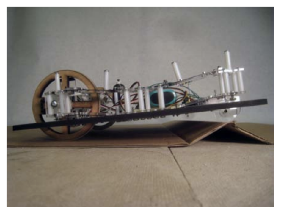
(a) Actual robot suspension.

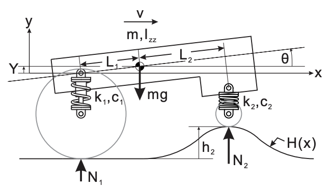
(b) Robot suspension model.

Figure 20.1: Mobile robot suspension

positions and velocities in both \(x\) and \(y\) at the rear and front wheels (assuming \(\theta\) is small) as \[\begin{aligned} &X_{1}=X-L_{1}, \quad\left(\dot{X}_{1}=v\right) \\ &X_{2}=X+L_{2}, \quad\left(\dot{X}_{2}=v\right) \\ &Y_{1}=Y-L_{1} \theta \\ &\dot{Y}_{1}=\dot{Y}-L_{1} \dot{\theta} \\ &Y_{2}=Y+L_{2} \theta \\ &\dot{Y}_{2}=\dot{Y}+L_{2} \dot{\theta} \end{aligned}\] where \(L_{1}\) and \(L_{2}\) are the distances to the system’s center of mass from the rear and front wheels. (Recall ’ refers to time derivative.) Note that we define \(Y=0\) as the height of the robot’s center of mass with both wheels in contact with flat ground and both springs at their unstretched and uncompressed lengths, i.e., when \(N_{1}=N_{2}=0\). Next, we determine the heights of the ground at the rear and front contact points as \[\begin{aligned} &h_{1}=H\left(X_{1}\right) \\ &h_{2}=H\left(X_{2}\right) \end{aligned}\] Similarly, the rates of change of the ground height at the rear and front are given by \[\begin{aligned} \frac{d h_{1}}{d t} &=\dot{h}_{1}=v \frac{d}{d x} H\left(X_{1}\right) \\ \frac{d h_{2}}{d t} &=\dot{h}_{2}=v \frac{d}{d x} H\left(X_{2}\right) \end{aligned}\] Note that we must multiply the spatial derivatives \(\frac{d H}{d x}\) by \(v=\frac{d X}{d t}\) to find the temporal derivatives.

While the wheels are in contact with the ground we can determine the normal forces at the rear and front from the constitutive equations for the springs and dampers as \[\begin{aligned} &N_{1}=k_{1}\left(h_{1}-Y_{1}\right)+c_{1}\left(\dot{h}_{1}-\dot{Y}_{1}\right) \\ &N_{2}=k_{2}\left(h_{2}-Y_{2}\right)+c_{2}\left(\dot{h}_{2}-\dot{Y}_{2}\right) \end{aligned}\] If either \(N_{1}\) or \(N_{2}\) is calculated from Equations \((20.5)\) to be less than or equal to zero, we can determine that the respective wheel has lost contact with the ground and stop the simulation, concluding loss of contact, i.e., failure.

Finally, we can determine the rates of change of the state from the linearized \((\cos \theta \approx 1\), \(\sin \theta \approx \theta\) ) equations of motion for the robot, given by Newton-Euler as \[\begin{aligned} \ddot{X} &=0, \quad \dot{X}=v, \quad X(0)=0, \\ \ddot{Y} &=-g+\frac{N_{1}+N_{2}}{m}, \quad \dot{Y}(0)=\dot{Y}_{0}, \quad Y(0)=Y_{0}, \\ \ddot{\theta} &=\frac{N_{2} L_{2}-N_{1} L_{1}}{I_{z z}}, \quad \dot{\theta}(0)=\dot{\theta}_{0}, \quad \theta(0)=\theta_{0}, \end{aligned}\] where \(m\) is the mass of the robot, and \(I_{z z}\) is the moment of inertia of the robot about an axis parallel to the \(Z\) axis passing through the robot’s center of mass.

In this unit we shall discuss the numerical procedures by which to integrate systems of ordinary differential equations such as \(\underline{(20.6)}\). This integration can then permit us to determine loss of contact and hence failure.