26.5: Tridiagonal Systems

While the cost of Gaussian elimination scales as \(n^{3}\) for a general \(n \times n\) linear system, there are instances in which the scaling is much weaker and hence the computational cost for a large problem is relatively low. A tridiagonal system is one such example. A tridigonal system is characterized by having nonzero entries only along the main diagonal and the immediate upper and lower diagonal, i.e.

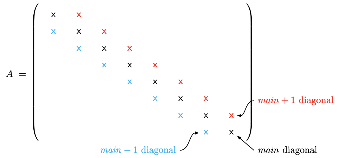
The immediate upper diagonal is called the super-diagonal and the immediate lower diagonal is called the sub-diagonal. A significant reduction in the computational cost is achieved by taking advantage of the sparsity of the tridiagonal matrix. That is, we omit addition and multiplication of a large number of zeros present in the matrix.

Let us apply Gaussian elimination to the \(n \times n\) tridiagonal matrix. In the first step, we compute the scaling factor (one FLOP), scale the second entry of the coefficient of the first row by the scaling factor (one FLOP), and add that to the second coefficient of the second row (one FLOP). (Note that we do not need to scale and add the first coefficient of the first equation to that of the second equation because we know it will vanish by construction.) We do not have to add the first equation to any other equations because the first coefficient of all other equations are zero. Moreover, note that the addition of the (scaled) first row to the second row does not introduce any new nonzero entry in the second row. Thus, the updated matrix has zeros above the super-diagonal and retains the tridiagonal structure of the original matrix (with the \((2,1)\) entry eliminated, of course); in particular, the updated \((n-1) \times(n-1)\) sub-block is again tridiagonal. We also modify the righthand side by multiplying the first entry by the scaling factor (one FLOP) and adding it to the second entry (one FLOP). Combined with the three FLOPs required for the matrix manipulation, the total cost for the first step is five FLOPs.

Similarly, in the second step, we use the second equation to eliminate the leading nonzero coefficient of the third equation. Because the structure of the problem is identical to the first one, this also requires five FLOPs. The updated matrix retain the tridiagonal structure in this elimination step and, in particular, the updated \((n-2) \times(n-2)\) sub-block is tridiagonal. Repeating the operation for \(n\) steps, the total cost for producing an upper triangular system (and the associated modified right-hand side) is \(5 n\) FLOPs. Note that the cost of Gaussian elimination for a tridiagonal system scales linearly with the problem size \(n\) : a dramatic improvement compared to \(\mathcal{O}\left(n^{3}\right)\) operations required for a general case.

At this point, we have produced an upper triangular system of the form

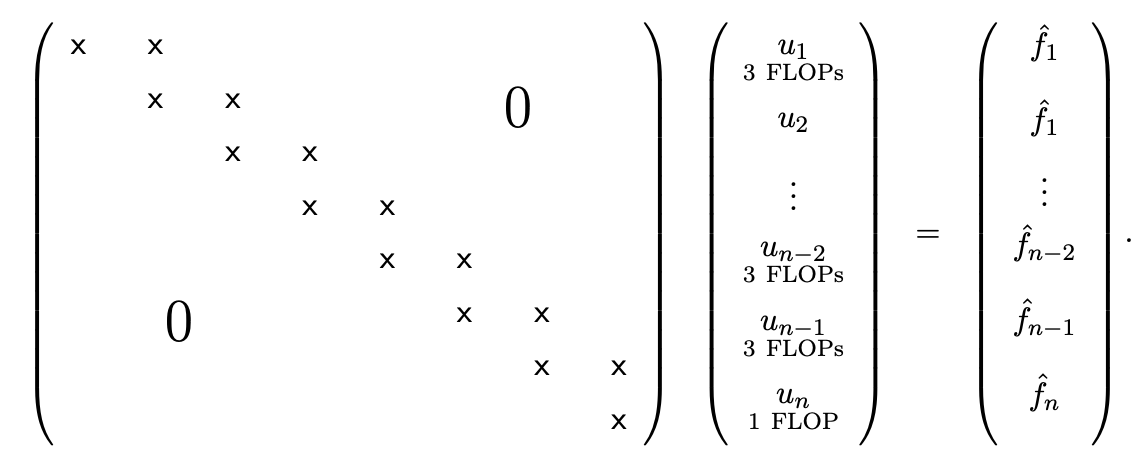
The system is said to be bidiagonal - or more precisely upper bidiagonal - as nonzero entries appear only on the main diagonal and the super-diagonal. (A matrix that has nonzero entries only on the main and sub-diagonal are also said to be bidiagonal; in this case, it would be lower bidiagonal.)

In the back substitution stage, we can again take advantage of the sparsity - in particular the bidiagonal structure - of our upper triangular system. As before, evaluation of \(u_{n}\) requires a simple division (one FLOP). The evaluation of \(u_{n-1}\) requires one scaled subtraction of \(u_{n}\) from the right-hand side (two FLOPs) and one division (one FLOP) for three total FLOPs. The structure is the same for the remaining \(n-2\) unknowns; the evaluating each entry takes three FLOPs. Thus, the total cost of back substitution for a bidiagonal matrix is \(3 n\) FLOPs. Combined with the cost of the Gaussian elimination for the tridiagonal matrix, the overall cost for solving a tridiagonal system is \(8 n\) FLOPs. Thus, the operation count of the entire linear solution procedure (Gaussian elimination and back substitution) scales linearly with the problem size for tridiagonal matrices.

We have achieved a significant reduction in computational cost for a tridiagonal system compared to a general case by taking advantage of the sparsity structure. In particular, the computational cost has been reduced from \(2 n^{3} / 3\) to \(8 n\). For example, if we wish to solve for the equilibrium displacement of a \(n=1000\) spring-mass system (which yields a tridiagonal system), we have reduced the number of operations from an order of a billion to a thousand. In fact, with the tridiagonal-matrix algorithm that takes advantage of the sparsity pattern, we can easily solve a spring-mass system with millions of unknowns on a desktop machine; this would certainly not be the case if the general Gaussian elimination algorithm is employed, which would require \(\mathcal{O}\left(10^{18}\right)\) operations.

While many problems in engineering require solution of a linear system with millions (or even billions) of unknowns, these systems are typically sparse. (While these systems are rarely tridiagonal, most of the entries of these matrices are zero nevertheless.) In the next chapter, we consider solution to more general sparse linear systems; just as we observed in this tridiagonal case, the key to reducing the computational cost for large sparse matrices - and hence making the computation tractable - is to study the nonzero pattern of the sparse matrix and design an algorithm that does not execute unnecessary operations.