28.1: The Matrix Vector Product

To illustrate some of the fundamental aspects of computations with sparse matrices we shall consider the calculation of the matrix vector product, \(w=A v\), for \(A\) a given \(n \times n\) sparse matrix as defined above and \(v\) a given \(n \times 1\) vector. (Note that we considering here the simpler forward problem, in which \(v\) is known and \(w\) unknown; in a later section we consider the more difficult "inverse" problem, in which \(w\) is known and \(v\) is unknown.)

Mental Model

We first consider a mental model which provides intuition as to how the sparse matrix vector product is calculated. We then turn to actual MATLAB implementation which is different in detail from the mental model but very similar in concept. There are two aspects to sparse matrices: how these matrices are stored (efficiently); and how these matrices are manipulated (efficiently). We first consider storage.

Storage

By definition our matrix \(A\) is mostly zeros and hence it would make no sense to store all the entries. Much better is to just store the \(\operatorname{nnz}(A)\) nonzero entries with the convention that all other entries are indeed zero. This can be done by storing the indices of the nonzero entries as well as the values, as indicated in (28.1). \[\left.\begin{array}{c} I(m), J(m), 1 \leq m \leq \mathrm{nnz}(A): \\ \text { indices } i=I(m), j=J(m) \\ \text { for which } A_{i j} \neq 0 \\ V_{A}(m), 1 \leq m \leq \mathrm{nnz}(A): \\ \text { value of } A_{I(m), J(m)} \end{array}\right\} \begin{gathered} \mathcal{O}(\mathrm{nnz}(A)) \text { storage } \\ \ll n^{2} \text { if sparse } \end{gathered}\] Here \(m\) is an index associated to each nonzero entry, \(I(m), J(m)\) are the indices of the \(m^{\text {th }}\) nonzero entry, and \(V_{A}(m)\) is the value of \(A\) associated with this index, \(V_{A}(m) \equiv A_{I(m), J(m)}\). Note that \(V_{A}\) is a vector and not a matrix. It is clear that if \(A\) is in fact dense then the scheme (28.1) actually requires more storage than the conventional non-sparse format since we store values of the indices as well as the values of the matrix; but for sparse matrices the scheme (28.1) can result in significant economies.

As a simple example we consider \(A=I\), the \(n \times n\) identity matrix, for which \(n \mathrm{nz}(A)=n\) - a very sparse matrix. Here our sparse storage scheme can be depicted as in (28.2).

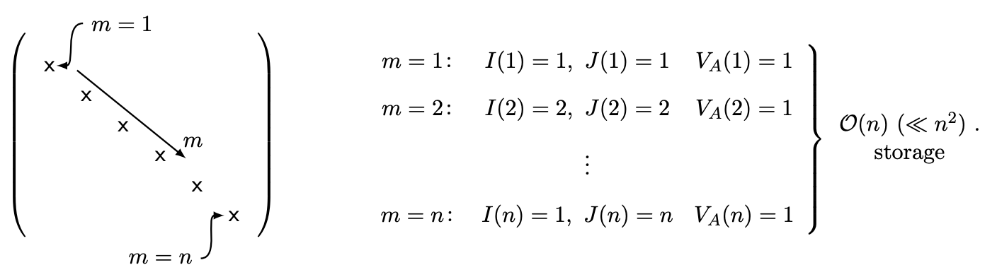
We note that the mapping between the index \(m\) and the nonzero entries of \(A\) is of course nonunique; in the above we identify \(m\) with the row (or equivalently, column) of the entry on the main diagonal, but we could equally well number backwards or "randomly."

Operations

We now consider the sparse matrix-vector product in terms of the storage scheme introduced above. In particular, we claim that \[\underbrace{w}_{\text {to find }}=A \underbrace{v}_{\text {given }}\] can be implemented as \[w=\operatorname{zeros}(n, 1)\] \[\begin{aligned} & \text { for } m=1: \operatorname{nnz}(A) \\ & w(I(m))=w(I(m))+V_{A}(m) \times v(J(m)) \end{aligned}\] end

We now discuss why this algorithm yields the desired result. We first note that for any \(i\) such that \(I(m) \neq i\) for any \(m\) - in other words, a row \(i\) of \(A\) which is entirely zero - \(w(i)\) should equal zero by the usual row interpretation of the matrix vector product: \(w(i)\) is the inner product between the \(i^{\text {th }}\) row of \(A\) - all zeros - and the vector \(v\), which vanishes for any \(v\). \[i \rightarrow\left(\begin{array}{ccccc} 0 & 0 & \cdots & 0 & 0 \\ & & & & \\ A & & \\ v \\ x \end{array}\right) \quad\left(\begin{array}{c} x \\ x \\ w \end{array}\right)=\left(\begin{array}{c} 0 \\ w \end{array}\right)\] On the other hand, for any \(i\) such that \(I(m)=i\) for some \(m\), \[w(i)=\sum_{j=1}^{n} A_{i j} v_{j}=\sum_{\substack{j=1 \\ A_{i j} \neq 0}}^{n} A_{i j} v_{j} .\] In both cases the sparse procedure yields the correct result and furthermore does not perform all the unnecessary operations associated with elements \(A_{i j}\) which are zero and which will clearly not contribute to the matrix vector product: zero rows of \(A\) are never visited; and in rows of \(A\) with nonzero entries only the nonzero columns are visited. We conclude that the operation count is \(\mathcal{O}(\mathrm{nnz}(A))\) which is much less than \(n^{2}\) if our matrix is indeed sparse.

We note that we have not necessarily used all possible sparsity since in addition to zeros in \(A\) there may also be zeros in \(v\); we may then not only disregard any row of \(A\) which are is zero but we may also disregard any column \(k\) of \(A\) for which \(v_{k}=0\). In practice in most MechE examples the sparsity in \(A\) is much more important to computational efficiency and arises much more often in actual practice than the sparsity in \(v\), and hence we shall not consider the latter further.

Matlab Implementation

It is important to recognize that sparse is an attribute associated not just with the matrix \(A\) in a linear algebra or mathematical sense but also an attribute in MATLAB (or other programming languages) which indicates a particular data type or class (or, in MATLAB, attribute). In situations in which confusion might occur we shall typically refer to the former simply as sparse and the latter as "declared" sparse. In general we will realize the computational savings associated with a mathematically sparse matrix \(A\) only if the corresponding MATLAB entity, A, is also declared sparse - it is the latter that correctly invokes the sparse storage and algorithms described in the previous section. (We recall here that the MATLAB implementation of sparse storage and sparse methods is conceptually similarly to our mental model described above but not identical in terms of details.)

Storage

We proceed by introducing a brief example which illustrates most of the necessary MATLAB functionality and syntax. In particular, the script

n = 5;
K = spalloc(n,n,3*n);
K(1,1) = 2; 
K(1,2) = -1; 
for i = 2:n-1 
    K(i,i) = 2; 
    K(i,i-1) = -1; 
    K(i,i+1) = -1; 
end 
K(n,n) = 1; 
K(n,n-1) = -1;

is_K_sparse = issparse(K)

K 

num_nonzeros_K = nnz(K)

spy(K) 

K_full = full(K) 

K_sparse_too = sparse(K_full)

yields the output

is_K_sparse = 
    1

K = (1,1)  2 
    (2,1) -1 
    (1,2) -1 
    (2,2)  2 
    (3,2) -1 
    (2,3) -1 
    (3,3)  2 
    (4,3) -1 
    (3,4) -1 
    (4,4)  2 
    (5,4) -1 
    (4,5) -1 
    (5,5)  1 
    
num_nonzeros_K =

Figure 28.1: Output of spy (K).

    13
K_full = 2 -1  0  0  0 
        -1  2 -1  0  0 
         0 -1  2 -1  0 
         0  0 -1  2 -1 
         0  0  0 -1  1
         
K_sparse_too = 
    (1,1)  2 
    (2,1) -1 
    (1,2) -1 
    (2,2)  2 
    (3,2) -1 
    (2,3) -1 
    (3,3)  2 
    (4,3) -1 
    (3,4) -1 
    (4,4)  2 
    (5,4) -1 
    (4,5) -1 
    (5,5)  1

as well as Figure \(28.1 .\)

We now explain the different parts in more detail:

First, \(\mathrm{M}=\operatorname{spalloc}(\mathrm{n} 1, \mathrm{n} 2, \mathrm{k})(i)\) creates a declared sparse array \(\mathrm{M}\) of size \(\mathrm{n} 1 \times \mathrm{n} 2\) with allocation for \(\mathrm{k}\) nonzero matrix entries, and then \((i i\) ) initializes the array M to all zeros. (If later in the script this allocation may be exceeded there is no failure or error, however efficiency will suffer as memory will not be as contiguously assigned.) In our case here, we anticipate that \(K\) will be tri-diagonal and hence there will be less than \(3 *\) nonzero entries.

Then we assign the elements of \(K\) - we create a simple tri-diagonal matrix associated with \(n=5\) springs in series. Note that although \(K\) is declared sparse we do not need to assign values according to any complicated sparse storage scheme: we assign and more generally refer to the elements of \(K\) with the usual indices, and the sparse storage bookkeeping is handled by MATLAB under the hood.

We can confirm that a matrix \(M\) is indeed (declared) sparse with issparse - issparse(M) returns a logical 1 if \(M\) is sparse and a logical 0 if \(M\) is not sparse. (In the latter case, we will not save on memory or operations.) As we discuss below, some MATLAB operations may accept sparse operands but under certain conditions return non-sparse results; it is often important to confirm with issparse that a matrix which is intended to be sparse is indeed (declared) sparse.

Now we display \(K\). We observe directly the sparse storage format described in the previous section: MATLAB displays effectively \(\left(I(m), J(m), V_{A}(m)\right)\) triplets (MATLAB does not display \(m\), which as we indicated is in any event an arbitrary label).

The MATLAB built-in function \(n n z(M)\) returns the number of nonzero entries in a matrix M. The MATLAB built-in function spy \((M)\) displays the \(n 1 \times\) n2 matrix M as a rectangular grid with (only) the nonzero entries displayed as blue filled circles - Figure \(28.1\) displays spy (K). In short, nnz and spy permit us to quantify the sparsity and structure, respectively, of a matrix \(M\).

The MATLAB built-in functions full and sparse create a full matrix from a (declared) sparse matrix and a (declared) sparse matrix from a full matrix respectively. Note however, that it is better to initialize a sparse matrix with spalloc rather than simply create a full matrix and then invoke sparse; the latter will require at least temporarily (but sometimes fatally) much more memory than the former.

There are many other sparse MATLAB built-in functions for performing various operations.

Operations

This section is very brief: once a matrix A is declared sparse, then the MATLAB statement \(\mathrm{w}=\mathrm{A} * \mathrm{v}\) will invoke the efficient sparse matrix vector product described above. In short, the (matrix) multiplication operator \(*\) recognizes that A is a (declared) sparse matrix object and then automatically invokes the correct/efficient "method" of interpretation and evaluation. Note in the most common application and in our case most relevant application the matrix A will be declared sparse, the vector v will be full (i.e., not declared sparse), and the output vector w will be full (i.e., not declared sparse). \({ }^{1}\) We emphasize that if the matrix A is mathematically sparse but not declared sparse then the MATLAB * operand will invoke the standard full matrix-vector multiply and we not realize the potential computational savings.

\({ }^{1}\) Note if the vector \(\mathrm{v}\) is also declared sparse then the result \(\mathrm{w}\) will be declared sparse as well.