29.4: Continuation and Homotopy

Often we are interested not in solving just a single nonlinear problem, but rather a family of nonlinear problems \(\boldsymbol{f}(\boldsymbol{Z} ; \mu)=\mathbf{0}\) with real parameter \(\mu\) which can take on a sequence of values \(\mu_{(1)}, \ldots, \mu_{(p)}\). Typically we supplement \(\boldsymbol{f}(\boldsymbol{Z} ; \mu)=0\) with some simple constraints or continuity conditions which select a particular solution from several possible solutions.

We then wish to ensure that, \((i)\) we are able to start out at all, often by transforming the initial problem for \(\mu=\mu_{(1)}\) (and perhaps also subsequent problems for \(\mu=\mu_{(i)}\) ) into a series of simpler problems (homotopy) and, (ii) once started, and as the parameter \(\mu\) is varied, we continue to converge to "correct" solutions as defined by our constraints and continuity conditions (continuation).

Parametrized Nonlinear Problems: A Single Parameter

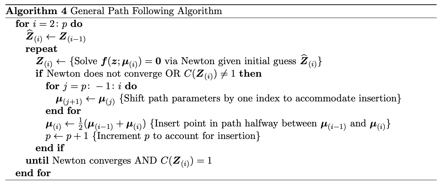
Given \(\boldsymbol{f}(\boldsymbol{Z} ; \mu)=0\) with real single parameter \(\mu\), we are typically interested in how our solution \(\boldsymbol{Z}\) changes as we change \(\mu\); in particular, we now interpret (à la the implicit function theorem) \(\boldsymbol{Z}\) as a function \(\boldsymbol{Z}(\mu)\). We can visualize this dependency by plotting \(Z\) (here \(n=1\) ) with respect to \(\mu\), giving us a bifurcation diagram of the problem, as depicted in Figure \(29.7\) for several common modes of behavior.

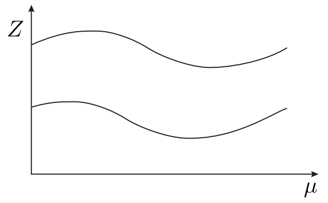
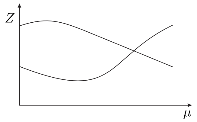
Figure 29.7(a) depicts two isolated solution branches with two, distinct real solutions over the whole range of \(\mu\). Figure 29.7(b) depicts two solution branches that converge at a singular point, where a change in \(\mu\) can drive the solution onto either of the two branches. Figure 29.7(c) depicts two solution branches that converge at a limit point, beyond which there is no solution.

(a) isolated branches

(b) singular point

(c) limit point

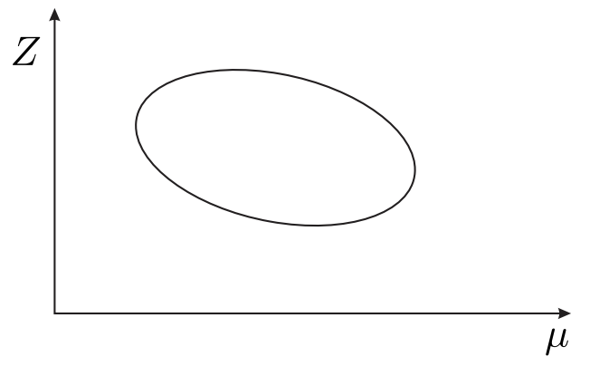
(d) isola

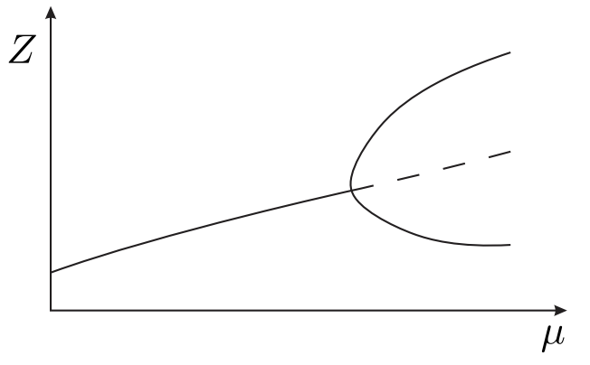
(e) pitchfork

Figure 29.7: Bifurcation Diagram: Several Common Modes of Behavior.

Figure 29.8: Simple mechanical linkage.

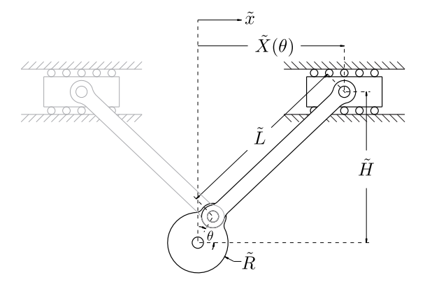
Figure 29.7(d) depicts an isola, an isolated interval of two solution branches with two limit points for endpoints. Figure \(29.7(\mathrm{e})\) depicts a single solution branch that "bifurcates" into several solutions at a pitchfork; pitchfork bifurcations often correspond to nonlinear dynamics that can display either stable (represented by solid lines in the figure) or unstable (represented by dotted lines) behavior, where stability refers to the ability of the state variable \(\boldsymbol{Z}\) to return to the solution when perturbed.

Note that, for all of the mentioned cases, when we reach a singular or limit point - characterized by the convergence of solution branches - the Jacobian becomes singular (non-invertible) and hence Newton breaks down unless supplemented by additional conditions.

Simple Example

We can develop an intuitive understanding of these different modes of behavior and corresponding bifurcation diagrams by considering a simple example.

We wish to analyze the simple mechanical linkage shown in Figure \(29.8\) by finding \(\widetilde{X}\) corresponding to an arbitrary \(\theta\) for given (constant) \(\widetilde{H}, \widetilde{R}\), and \(\widetilde{L}\). In this example, then, \(\theta\) corresponds to the earlier discussed generic parameter \(\mu\).

We can find an analytical solution for \(\widetilde{X}(\theta ; \widetilde{R}, \widetilde{H}, \widetilde{L})\) by solving the geometric constraint \[(\widetilde{X}-\widetilde{R} \cos \theta)^{2}+(\widetilde{H}-\widetilde{R} \sin \theta)^{2}=\widetilde{L}^{2},\] which defines the distance between the two joints as \(\widetilde{L}\). This is clearly a nonlinear equation, owing to the quadratic term in \(\tilde{x}\). We can eliminate one parameter from the equation by non-dimensionalizing with respect to \(\widetilde{L}\), giving us \[(X-R \cos \theta)^{2}+(H-R \sin \theta)^{2}=1,\] where \(X=\frac{\tilde{X}}{\tilde{L}}, R=\frac{\tilde{R}}{\tilde{L}}\), and \(H=\frac{\tilde{H}}{\tilde{L}}\). Expanding and simplifying, we get \[a X^{2}+b X+c \equiv f(X ; \theta ; R, H)=0,\] where \(a=1, b=-2 R \cos \theta\), and \(c=R^{2}+H^{2}-2 H R \sin \theta-1\). A direct application of the quadratic formula then gives us the two roots \[\begin{aligned} &X_{+}=\frac{-b+\sqrt{b^{2}-4 a c}}{2 a}, \\ &X_{-}=\frac{-b-\sqrt{b^{2}-4 a c}}{2 a}, \end{aligned}\] which may be real or complex.

We observe three categories for the number of solutions to our quadratic equation depending on the value of the discriminant \(\Delta(\theta ; R, H) \equiv b^{2}-4 a c\). First, if \(\Delta<0, \sqrt{\Delta}\) is imaginary and there is no (real) solution. An example is the case in which \(\widetilde{H}>\widetilde{L}+\widetilde{R}\). Second, if \(\Delta=0\), there is exactly one solution, \(X=\frac{-b}{2 a}\). An example is the case in which \(\widetilde{H}=\widetilde{L}+\widetilde{R}\) and \(\theta=\frac{\pi}{2}\). Third, if \(\Delta>0\), there are two distinct solutions, \(X_{+}\)and \(X_{-}\); an example is shown in Figure 29.8. Note that with our simple crank example we can obtain all the cases of Figure 29.7 except Figure 29.7(e).

We note that the case of two distinct solutions is new - our linear systems of equations (for the univariate case, \(f(x)=A x-b)\) had either no solution ( \(A=0, b \neq 0\); line parallel to \(x\) axis), exactly one solution ( \(A \neq 0\); line intersecting \(x\) axis), or an infinite number of solutions \((A=0\), \(b=0\); line on \(x\) axis). Nonlinear equations, on the other hand, have no such restrictions. They can have no solution, one solution, two solutions (as in our quadratic case above), three solutions (e.g., a cubic equation) - any finite number of solutions, depending on the nature of the particular function \(f(z)\) - or an infinite number of solutions (e.g., a sinusoidal equation). For example, if \(f(z)\) is an \(n^{\text {th }}\)-order polynomial, there could be anywhere from zero to \(n\) (real) solutions, depending on the values of the \(n+1\) parameters of the polynomial.

It is important to note, for the cases in which there are two, distinct solution branches corresponding to \(X_{+}\)and \(X_{-}\), that, as we change the \(\theta\) of the crank, it would be physically impossible to jump from one branch to the other - unless we stopped the mechanism, physically disassembled it, and then reassembled it as a mirror image of itself. Thus for the physically relevant solution we must require a continuity condition, or equivalently a constraint that requires \(\left|X\left(\theta_{(i)}\right)-X\left(\theta_{(i-1)}\right)\right|\) not too large or perhaps \(X\left(\theta_{(i)}\right) X\left(\theta_{(i-1)}\right)>0\); here \(\theta_{(i)}\) and \(\theta_{(i-1)}\) are successive parameters in our family of solutions.

In the Introduction, Section 29.1, we provide an example of a linkage with two degrees of freedom. In this robot arm example the parameter \(\boldsymbol{\mu}\) is given by \(\boldsymbol{X}\), the desired position of the end effector.

Path Following: Continuation

As already indicated, as we vary our parameter \(\mu\) (corresponding to \(\theta\) in the crank example), we must reflect any constraint (such as, in the crank example, no "re-assembly") in our numerical approach to ensure that the solution to which we converge is indeed the "correct" one. One approach is through an appropriate choice of initial guess. Inherent in this imperative is an opportunity - we can exploit information about our previously converged solution not only to keep us on the appropriate solution branch, but also to assist continued (rapid) convergence of the Newton iteration.

We denote our previously converged solution to \(f(Z ; \mu)=0\) as \(Z\left(\mu_{(i-1)}\right)\) (we consider here the univariate case). We wish to choose an initial guess \(\widehat{Z}\left(\mu_{(i)}\right)\) to converge to (a nearby root) \(Z\left(\mu_{(i)}\right)=Z\left(\mu_{(i-1)}+\delta \mu\right)\) for some step \(\delta \mu\) in \(\mu\). The simplest approach is to use the previously converged solution itself as our initial guess for the next step, \[\widehat{Z}\left(\mu_{(i)}\right)=Z\left(\mu_{(i-1)}\right) .\] This is often sufficient for small changes \(\delta \mu\) in \(\mu\) and it is certainly the simplest approach.

We can improve our initial guess if we use our knowledge of the rate of change of \(Z(\mu)\) with respect to \(\mu\) to help us extrapolate, to wit \[\widehat{Z}\left(\mu_{(i)}\right)=Z\left(\mu_{(i-1)}\right)+\frac{\mathrm{d} Z}{\mathrm{~d} \mu} \delta \mu .\] We can readily calculate \(\frac{\mathrm{d} Z}{\mathrm{~d} \mu}\) as \[\frac{\mathrm{d} Z}{\mathrm{~d} \mu}=\frac{-\frac{\partial f}{\partial \mu}}{\frac{\partial f}{\partial z}}\] since \[f(Z(\mu) ; \mu)=0 \Rightarrow \frac{\mathrm{d} f}{\mathrm{~d} \mu}(Z(\mu) ; \mu) \equiv \frac{\partial f}{\partial z} \frac{\mathrm{d} Z}{\mathrm{~d} \mu}+\frac{\partial f}{\partial \mu} \frac{\mathrm{d} f^{\prime}}{d \mu}=0 \Rightarrow \frac{\mathrm{d} Z}{\mathrm{~d} \mu}=\frac{-\frac{\partial f}{\partial \mu}}{\frac{\partial f}{\partial z}}\] by the chain rule.

Cold Start: Homotopy

In many cases, given a previous solution \(Z\left(\mu_{(i-1)}\right)\), we can use either of equations (29.63) or (29.64) to arrive at an educated guess \(\widehat{Z}\left(\mu_{(i)}\right)\) for the updated parameter \(\mu_{(i)}\). If we have no previous solution, however, (e.g., \(i=1\) ) or our continuation techniques fail, we need some other means of generating an initial guess \(\widehat{Z}\left(\mu_{(i)}\right)\) that will be sufficiently good to converge to a correct solution.

A common approach to the "cold start" problem is to transform the original nonlinear problem \(f\left(Z\left(\mu_{(i)}\right) ; \mu_{(i)}\right)=0\) into a form \(\tilde{f}\left(Z\left(\mu_{(i)}, t\right) ; \mu_{(i)}, t\right)=0\), i.e., we replace \(f\left(Z ; \mu_{(i)}\right)=0\) with \(\tilde{f}\left(\widetilde{Z} ; \mu_{(i)}, t\right)=0\). Here \(t\) is an additional, artificial, continuation parameter such that, when \(t=0\), the solution of the nonlinear problem \[\tilde{f}\left(\widetilde{Z}\left(\mu_{(i)}, t=0\right) ; \mu_{(i)}, t=0\right)=0\] is relatively simple (e.g., linear) or, perhaps, coincides with a preceding, known solution, and, when \(t=1\), \[\tilde{f}\left(z ; \mu_{(i)}, t=1\right)=f\left(z ; \mu_{(i)}\right)\] such that \(\tilde{f}\left(\tilde{Z}\left(\mu_{(i)}, t=1\right) ; \mu_{(i)}, t=1\right)=0\) implies \(f\left(\tilde{Z}\left(\mu_{(i)}\right) ; \mu_{(i)}\right)=0\) and hence \(Z\left(\mu_{(i)}\right)\) (the desired solution \()=\widetilde{Z}\left(\mu_{(i)}, t=1\right)\).

We thus transform the "cold start" problem to a continuation problem in the artificial parameter \(t\) as \(t\) is varied from 0 to 1 with a start of its own (when \(t=0\) ) made significantly less "cold" by its - by construction - relative simplicity, and an end (when \(t=1\) ) that brings us smoothly to the solution of the original "cold start" problem.

As an example, we could replace the crank function \(f\) of \((29.61)\) with a function \(\tilde{f}(X ; \theta, t ; R, H)=\) at \(X^{2}+b X+c\) such that for \(t=0\) the problem is linear and the solution readily obtained.

General Path Approach: Many Parameters

We consider now an \(n\)-vector of functions \[\boldsymbol{f}(\boldsymbol{z} ; \boldsymbol{\mu})=\left(\begin{array}{llll} f_{1}(\boldsymbol{z} ; \boldsymbol{\mu}) & f_{2}(\boldsymbol{z} ; \boldsymbol{\mu}) & \ldots & f_{n}(\boldsymbol{z} ; \boldsymbol{\mu}) \end{array}\right)^{\mathrm{T}}\] that depends on an \(n\)-vector of unknowns \(\boldsymbol{z}\) \[\boldsymbol{z}=\left(\begin{array}{llll} z_{1} & z_{2} & \ldots & z_{n} \end{array}\right)^{\mathrm{T}}\] and a parameter \(\ell\)-vector \(\boldsymbol{\mu}\) (independent of \(\boldsymbol{z}\) ) \[\boldsymbol{\mu}=\left(\begin{array}{llll} \mu_{1} & \mu_{2} & \cdots & \mu_{\ell} \end{array}\right)^{\mathrm{T}} .\] We also introduce an inequality constraint function \[C(\boldsymbol{Z})= \begin{cases}1 & \text { if constraint satisfied } \\ 0 & \text { if constraint not satisfied }\end{cases}\] Note this is not a constraint on \(\boldsymbol{z}\) but rather a constraint on the (desired) root \(\boldsymbol{Z}\). Then, given \(\boldsymbol{\mu}\), we look for \(\boldsymbol{Z}=\left(\begin{array}{llll}Z_{1} & Z_{2} & \ldots & Z_{n}\end{array}\right)^{\mathrm{T}}\) such that \[\left\{\begin{array}{l} \boldsymbol{f}(\boldsymbol{Z} ; \boldsymbol{\mu})=\mathbf{0} \\ C(\boldsymbol{Z})=1 \end{array}\right.\] In words, \(\boldsymbol{Z}\) is a solution of \(n\) nonlinear equations in \(n\) unknowns subject which satisfies the constraint \(C\).

Now we consider a path or "trajectory" - a sequence of \(p\) parameter vectors \(\boldsymbol{\mu}_{(1)}, \ldots, \boldsymbol{\mu}_{(p)}\). We wish to determine \(\boldsymbol{Z}_{(i)}, 1 \leq i \leq p\), such that \[\left\{\begin{array}{l} \boldsymbol{f}\left(\boldsymbol{Z}_{(i)} ; \boldsymbol{\mu}_{(i)}\right)=\mathbf{0} \\ C\left(\boldsymbol{Z}_{(i)}\right)=1 \end{array}\right.\] We assume that \(\boldsymbol{Z}_{(1)}\) is known and that \(\boldsymbol{Z}_{(2)}, \ldots, \boldsymbol{Z}_{(p)}\) remain to be determined. We can expect, then, that as long as consecutive parameter vectors \(\boldsymbol{\mu}_{(i-1)}\) and \(\boldsymbol{\mu}_{(i)}\) are sufficiently close, we should be able to use our continuation techniques equations \((29.63)\) or \((29.64)\) to converge to a correct (i.e., satisfying \(C\left(\boldsymbol{Z}_{(i)}\right)=1\) ) solution \(\boldsymbol{Z}_{(i)}\). If, however, \(\boldsymbol{\mu}_{(i-1)}\) and \(\boldsymbol{\mu}_{(i)}\) are not sufficiently close, our continuation techniques will not be sufficient (i.e. we will fail to converge to a solution at all or we will fail to converge to a solution satisfying \(C\) ) and we will need to apply a - we hope more fail-safe homotopy.

We can thus combine our continuation and homotopy frameworks into a single algorithm. One such approach is summarized in Algorithm 4. The key points of this algorithm are that \((i)\) we are using the simple continuation approach given by equation (29.63) (i.e., using the previous solution as the initial guess for the current problem), and (ii) we are using a bisection-type homotopy that, each time Newton fails to converge to a correct solution, inserts a new point in the trajectory halfway between the previous correct solution and the failed point. The latter, in the language of homotopy, can be expressed as \[\tilde{\boldsymbol{f}}\left(\boldsymbol{z} ; \boldsymbol{\mu}_{(i)}, t\right)=\boldsymbol{f}\left(\boldsymbol{z} ;(1-t) \boldsymbol{\mu}_{(i-1)}+t \boldsymbol{\mu}_{(i)}\right)\] with \(t=0.5\) for the inserted point.

Although there are numerous other approaches to non-convergence in addition to Algorithm 4 , such as relaxed Newton - in which Newton provides the direction for the update, but then we take just some small fraction of the proposed step - Algorithm 4 is included mainly for its generality, simplicity, and apparent robustness.