12.5: Absolute Motion Analysis
- Page ID
- 111401

\( \newcommand{\vecs}[1]{\overset { \scriptstyle \rightharpoonup} {\mathbf{#1}} } \)
\( \newcommand{\vecd}[1]{\overset{-\!-\!\rightharpoonup}{\vphantom{a}\smash {#1}}} \)
\( \newcommand{\id}{\mathrm{id}}\) \( \newcommand{\Span}{\mathrm{span}}\)
( \newcommand{\kernel}{\mathrm{null}\,}\) \( \newcommand{\range}{\mathrm{range}\,}\)
\( \newcommand{\RealPart}{\mathrm{Re}}\) \( \newcommand{\ImaginaryPart}{\mathrm{Im}}\)
\( \newcommand{\Argument}{\mathrm{Arg}}\) \( \newcommand{\norm}[1]{\| #1 \|}\)
\( \newcommand{\inner}[2]{\langle #1, #2 \rangle}\)
\( \newcommand{\Span}{\mathrm{span}}\)
\( \newcommand{\id}{\mathrm{id}}\)
\( \newcommand{\Span}{\mathrm{span}}\)
\( \newcommand{\kernel}{\mathrm{null}\,}\)
\( \newcommand{\range}{\mathrm{range}\,}\)
\( \newcommand{\RealPart}{\mathrm{Re}}\)
\( \newcommand{\ImaginaryPart}{\mathrm{Im}}\)
\( \newcommand{\Argument}{\mathrm{Arg}}\)
\( \newcommand{\norm}[1]{\| #1 \|}\)
\( \newcommand{\inner}[2]{\langle #1, #2 \rangle}\)
\( \newcommand{\Span}{\mathrm{span}}\) \( \newcommand{\AA}{\unicode[.8,0]{x212B}}\)
\( \newcommand{\vectorA}[1]{\vec{#1}} % arrow\)
\( \newcommand{\vectorAt}[1]{\vec{\text{#1}}} % arrow\)
\( \newcommand{\vectorB}[1]{\overset { \scriptstyle \rightharpoonup} {\mathbf{#1}} } \)
\( \newcommand{\vectorC}[1]{\textbf{#1}} \)
\( \newcommand{\vectorD}[1]{\overrightarrow{#1}} \)
\( \newcommand{\vectorDt}[1]{\overrightarrow{\text{#1}}} \)
\( \newcommand{\vectE}[1]{\overset{-\!-\!\rightharpoonup}{\vphantom{a}\smash{\mathbf {#1}}}} \)
\( \newcommand{\vecs}[1]{\overset { \scriptstyle \rightharpoonup} {\mathbf{#1}} } \)
\( \newcommand{\vecd}[1]{\overset{-\!-\!\rightharpoonup}{\vphantom{a}\smash {#1}}} \)
\(\newcommand{\avec}{\mathbf a}\) \(\newcommand{\bvec}{\mathbf b}\) \(\newcommand{\cvec}{\mathbf c}\) \(\newcommand{\dvec}{\mathbf d}\) \(\newcommand{\dtil}{\widetilde{\mathbf d}}\) \(\newcommand{\evec}{\mathbf e}\) \(\newcommand{\fvec}{\mathbf f}\) \(\newcommand{\nvec}{\mathbf n}\) \(\newcommand{\pvec}{\mathbf p}\) \(\newcommand{\qvec}{\mathbf q}\) \(\newcommand{\svec}{\mathbf s}\) \(\newcommand{\tvec}{\mathbf t}\) \(\newcommand{\uvec}{\mathbf u}\) \(\newcommand{\vvec}{\mathbf v}\) \(\newcommand{\wvec}{\mathbf w}\) \(\newcommand{\xvec}{\mathbf x}\) \(\newcommand{\yvec}{\mathbf y}\) \(\newcommand{\zvec}{\mathbf z}\) \(\newcommand{\rvec}{\mathbf r}\) \(\newcommand{\mvec}{\mathbf m}\) \(\newcommand{\zerovec}{\mathbf 0}\) \(\newcommand{\onevec}{\mathbf 1}\) \(\newcommand{\real}{\mathbb R}\) \(\newcommand{\twovec}[2]{\left[\begin{array}{r}#1 \\ #2 \end{array}\right]}\) \(\newcommand{\ctwovec}[2]{\left[\begin{array}{c}#1 \\ #2 \end{array}\right]}\) \(\newcommand{\threevec}[3]{\left[\begin{array}{r}#1 \\ #2 \\ #3 \end{array}\right]}\) \(\newcommand{\cthreevec}[3]{\left[\begin{array}{c}#1 \\ #2 \\ #3 \end{array}\right]}\) \(\newcommand{\fourvec}[4]{\left[\begin{array}{r}#1 \\ #2 \\ #3 \\ #4 \end{array}\right]}\) \(\newcommand{\cfourvec}[4]{\left[\begin{array}{c}#1 \\ #2 \\ #3 \\ #4 \end{array}\right]}\) \(\newcommand{\fivevec}[5]{\left[\begin{array}{r}#1 \\ #2 \\ #3 \\ #4 \\ #5 \\ \end{array}\right]}\) \(\newcommand{\cfivevec}[5]{\left[\begin{array}{c}#1 \\ #2 \\ #3 \\ #4 \\ #5 \\ \end{array}\right]}\) \(\newcommand{\mattwo}[4]{\left[\begin{array}{rr}#1 \amp #2 \\ #3 \amp #4 \\ \end{array}\right]}\) \(\newcommand{\laspan}[1]{\text{Span}\{#1\}}\) \(\newcommand{\bcal}{\cal B}\) \(\newcommand{\ccal}{\cal C}\) \(\newcommand{\scal}{\cal S}\) \(\newcommand{\wcal}{\cal W}\) \(\newcommand{\ecal}{\cal E}\) \(\newcommand{\coords}[2]{\left\{#1\right\}_{#2}}\) \(\newcommand{\gray}[1]{\color{gray}{#1}}\) \(\newcommand{\lgray}[1]{\color{lightgray}{#1}}\) \(\newcommand{\rank}{\operatorname{rank}}\) \(\newcommand{\row}{\text{Row}}\) \(\newcommand{\col}{\text{Col}}\) \(\renewcommand{\row}{\text{Row}}\) \(\newcommand{\nul}{\text{Nul}}\) \(\newcommand{\var}{\text{Var}}\) \(\newcommand{\corr}{\text{corr}}\) \(\newcommand{\len}[1]{\left|#1\right|}\) \(\newcommand{\bbar}{\overline{\bvec}}\) \(\newcommand{\bhat}{\widehat{\bvec}}\) \(\newcommand{\bperp}{\bvec^\perp}\) \(\newcommand{\xhat}{\widehat{\xvec}}\) \(\newcommand{\vhat}{\widehat{\vvec}}\) \(\newcommand{\uhat}{\widehat{\uvec}}\) \(\newcommand{\what}{\widehat{\wvec}}\) \(\newcommand{\Sighat}{\widehat{\Sigma}}\) \(\newcommand{\lt}{<}\) \(\newcommand{\gt}{>}\) \(\newcommand{\amp}{&}\) \(\definecolor{fillinmathshade}{gray}{0.9}\)Absolute motion analysis is one method used to analyze bodies undergoing general planar motion. General planar motion is motion where bodies can both translate and rotate at the same time. Besides absolute motion analysis, the alternative is relative motion analysis. Either method can be used for any general planar motion problem, but one method may be significantly easier to apply for a given situation.
Absolute motion analysis will require calculus, and is generally faster for simple problems and problems where only the velocities (and not accelerations) are required. Relative motion analysis will not require calculus, but does necessitate using multiple coordinate systems; it is generally easier to use for more complex problems and problems where velocities and accelerations are being analyzed.
Utilizing Absolute Motion Analysis:
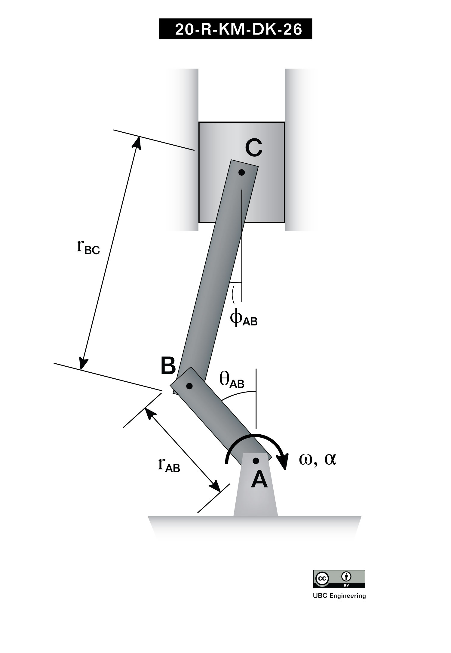
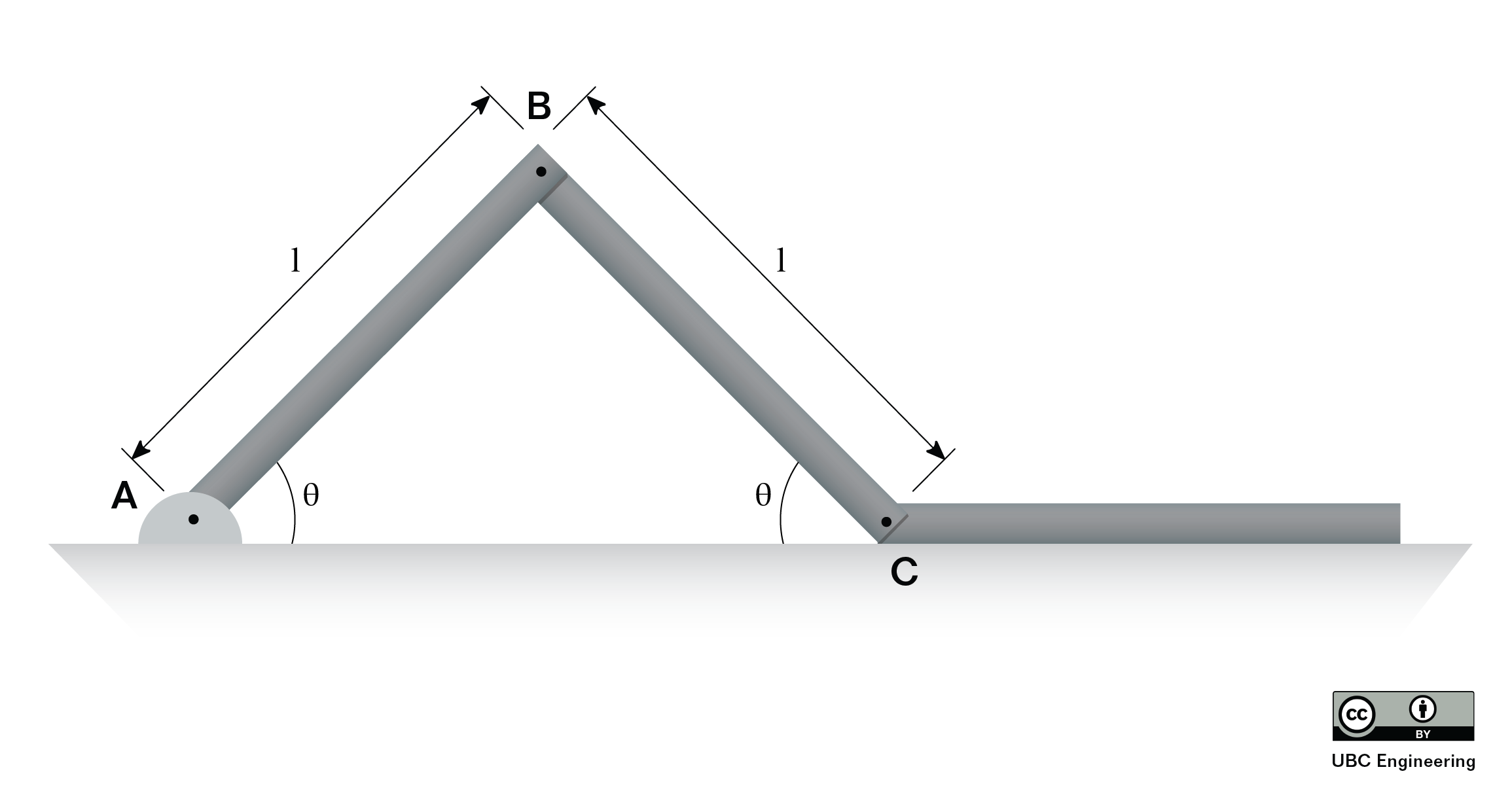
To start our discussion on absolute motion analysis, we are going to imagine a simple robotic arm such as the one below. In this arm, we have two arm sections of fixed length with motors causing rotations at joint A and joint B.
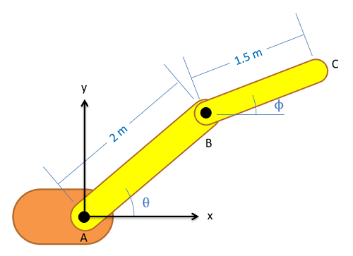
The first step in absolute motion analysis is come up with a set of equations describing the position of some point of interest. In this case we will be looking at the position of the end effector of the arm at point C, and we will write an equation for the \(x\) position and the \(y\) position of this point with respect to the fixed origin point at A. In these equations, anything that is a constant (such as the length of the arm pieces) can be put in as a number, but anything that will change, such as angles \(\theta\) and \(\phi\), will need to remain as variables in these equations even if they are known at the moment. Using the values in the diagram, we would wind up with the following two position equations.
\begin{align} x \text{-position:} \quad &\, x_C = 2 \cos (\theta) + 1.5 \cos (\phi) \\[5pt] y \text{-position:} \quad &\, y_C = 2 \sin (\theta) + 1.5 \sin (\phi) \end{align}
To find the velocity of point C in the \(x\) and \(y\) directions, we simply need to take the derivatives of the position equations. The velocity equations for our robotic arm are below.
\begin{align} x \text{-velocity:} \quad &\, v_{x \ C} = -2 \sin (\theta) \ \dot{\theta} - 1.5 \sin (\phi) \ \dot{\phi}\\[5pt] y \text{-velocity:} \quad &\, v_{y \ C} = 2 \cos (\theta) \ \dot{\theta} + 1.5 \cos (\phi) \ \dot{\phi} \end{align}
To find the acceleration of point C in the \(x\) and \(y\) directions, we simply need to take the derivatives of the velocity equations. The acceleration equations for our robotic arm in the \(x\) and \(y\) directions are shown below.
\begin{align} x \text{ acceleration:} \quad &\, a_{x \ C} = -2 \cos (\theta) \ \dot{\theta}^2 - 2 \sin (\theta) \ \ddot{\theta} - 1.5 \cos (\phi) \ \dot{\phi}^2 - 1.5 \sin (\phi) \ \ddot{\phi} \\[5pt] y \text{ acceleration:} \quad &\, a_{y \ C} = -2 \sin (\theta) \ \dot{\theta}^2 + 2 \cos (\theta) \ \ddot{\theta} - 1.5 \sin (\phi) \ \dot{\phi}^2 + 1.5 \cos (\phi) \ \ddot{\phi} \end{align}
Once we have the velocity and acceleration equations, we can start solving for any unknowns. If we have known angular velocities and accelerations (\(\dot{\theta}\), \(\ddot{\theta}\), \(\dot{\phi}\), and \(\ddot{\phi}\)) we can plug those in to find the velocity and acceleration vectors for the end effector. In other instances, we may known the desired motion of the end effector (\(v_{xC}\), \(v_{yC}\), \(a_{xC}\), and \(a_{yC}\)) and will have to plug those values into the equations to solve for unknowns such as \(\dot{\theta}\) and so on.
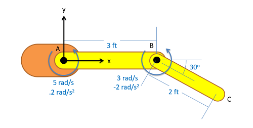
The robotic arm shown below has a fixed orange base at A and fixed-length members AB and BC. Motors at A and B allow for rotational motion at the joints. Based on the angular velocities and accelerations shown at each joint, determine the velocity and the acceleration of the end effector at C.
- Solution
-
Video \(\PageIndex{2}\): Worked solution to example problem \(\PageIndex{1}\), provided by Dr. Majid Chatsaz. YouTube source: https://youtu.be/ZBj17t8mhZc.
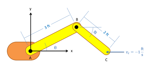
The robotic arm from the previous problem is in the configuration shown below. Assume that \(\theta\) is currently 30 degrees and that point C currently lies along the \(x\) axis. If we want the end effector at C to travel 1 ft/s in the negative \(x\)-direction, what should the angular velocities be at joints A and B?
- Solution
-
Video \(\PageIndex{3}\): Worked solution to example problem \(\PageIndex{2}\), provided by Dr. Majid Chatsaz. YouTube source: https://youtu.be/O5mtTTpK1RQ.
A ladder is propped up against a wall as shown below. If the base of the ladder is sliding out at a speed of 2 m/s, what is the speed of the top of the ladder?
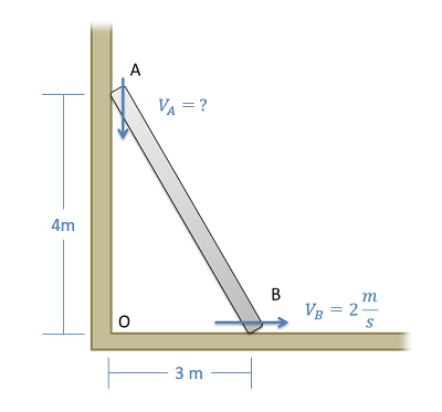
- Solution
-
Video \(\PageIndex{4}\): Worked solution to example problem \(\PageIndex{3}\), provided by Dr. Majid Chatsaz. YouTube source: https://youtu.be/fOfEaFUiDZI.
The crank-rocker mechanism as shown below consists of a crank with a radius of 0.5 meters rotating about its fixed center at C, at a constant rate of 2 rad/s clockwise. Rocker AB is fixed at its base at A and connects to point B along the edge of the crank. The pin at point B can slide along a frictionless slot in AB. In the current state, what is the angular velocity of rocker AB?
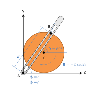
- Solution
-
Video \(\PageIndex{5}\): Worked solution to example problem \(\PageIndex{4}\), provided by Dr. Majid Chatsaz. YouTube source: https://youtu.be/DydbOzigdpU.
Question 5:
Determine the angular velocities and angular accelerations of links AB and BC if end D has a velocity of v=3m/s to the right and an acceleration of a=1m/s2 to the left. Link AB and BC both have a length l=0.5m and the angle is given as θ=60deg.
Solution:
Question 6:
Two linkages AB and BC are pinned together. Linkage AB is pinned at A meanwhile linkage BC can only slide horizontally at C. If VC=1 m/s , what is the relative velocity of B with respect to C ( V(B/C))? Assume the linkages are of equal length l=1m and at an angle of θ=30 deg with the horizontal.
Solution:
Question 7:
Students are attempting to create a lift to raise their model car. The lift is assembled with two linkages, link AB and link BC, as seen in the picture shown. If the links have length lAB=0.2 m and lBC=0.4 m, determine the velocity and acceleration of the lift at the instant where the angular velocity of AB is ωAB=-5 rad/s and the angular acceleration of AB is αAB=-7 rad/s2. Take the angles to be θ=30 deg and ϕ=20 deg.