
16.5: Viscous Damped Harmonic Forced Vibrations
- Page ID
- 111436

\( \newcommand{\vecs}[1]{\overset { \scriptstyle \rightharpoonup} {\mathbf{#1}} } \)
\( \newcommand{\vecd}[1]{\overset{-\!-\!\rightharpoonup}{\vphantom{a}\smash {#1}}} \)
\( \newcommand{\id}{\mathrm{id}}\) \( \newcommand{\Span}{\mathrm{span}}\)
( \newcommand{\kernel}{\mathrm{null}\,}\) \( \newcommand{\range}{\mathrm{range}\,}\)
\( \newcommand{\RealPart}{\mathrm{Re}}\) \( \newcommand{\ImaginaryPart}{\mathrm{Im}}\)
\( \newcommand{\Argument}{\mathrm{Arg}}\) \( \newcommand{\norm}[1]{\| #1 \|}\)
\( \newcommand{\inner}[2]{\langle #1, #2 \rangle}\)
\( \newcommand{\Span}{\mathrm{span}}\)
\( \newcommand{\id}{\mathrm{id}}\)
\( \newcommand{\Span}{\mathrm{span}}\)
\( \newcommand{\kernel}{\mathrm{null}\,}\)
\( \newcommand{\range}{\mathrm{range}\,}\)
\( \newcommand{\RealPart}{\mathrm{Re}}\)
\( \newcommand{\ImaginaryPart}{\mathrm{Im}}\)
\( \newcommand{\Argument}{\mathrm{Arg}}\)
\( \newcommand{\norm}[1]{\| #1 \|}\)
\( \newcommand{\inner}[2]{\langle #1, #2 \rangle}\)
\( \newcommand{\Span}{\mathrm{span}}\) \( \newcommand{\AA}{\unicode[.8,0]{x212B}}\)
\( \newcommand{\vectorA}[1]{\vec{#1}} % arrow\)
\( \newcommand{\vectorAt}[1]{\vec{\text{#1}}} % arrow\)
\( \newcommand{\vectorB}[1]{\overset { \scriptstyle \rightharpoonup} {\mathbf{#1}} } \)
\( \newcommand{\vectorC}[1]{\textbf{#1}} \)
\( \newcommand{\vectorD}[1]{\overrightarrow{#1}} \)
\( \newcommand{\vectorDt}[1]{\overrightarrow{\text{#1}}} \)
\( \newcommand{\vectE}[1]{\overset{-\!-\!\rightharpoonup}{\vphantom{a}\smash{\mathbf {#1}}}} \)
\( \newcommand{\vecs}[1]{\overset { \scriptstyle \rightharpoonup} {\mathbf{#1}} } \)
\( \newcommand{\vecd}[1]{\overset{-\!-\!\rightharpoonup}{\vphantom{a}\smash {#1}}} \)
\(\newcommand{\avec}{\mathbf a}\) \(\newcommand{\bvec}{\mathbf b}\) \(\newcommand{\cvec}{\mathbf c}\) \(\newcommand{\dvec}{\mathbf d}\) \(\newcommand{\dtil}{\widetilde{\mathbf d}}\) \(\newcommand{\evec}{\mathbf e}\) \(\newcommand{\fvec}{\mathbf f}\) \(\newcommand{\nvec}{\mathbf n}\) \(\newcommand{\pvec}{\mathbf p}\) \(\newcommand{\qvec}{\mathbf q}\) \(\newcommand{\svec}{\mathbf s}\) \(\newcommand{\tvec}{\mathbf t}\) \(\newcommand{\uvec}{\mathbf u}\) \(\newcommand{\vvec}{\mathbf v}\) \(\newcommand{\wvec}{\mathbf w}\) \(\newcommand{\xvec}{\mathbf x}\) \(\newcommand{\yvec}{\mathbf y}\) \(\newcommand{\zvec}{\mathbf z}\) \(\newcommand{\rvec}{\mathbf r}\) \(\newcommand{\mvec}{\mathbf m}\) \(\newcommand{\zerovec}{\mathbf 0}\) \(\newcommand{\onevec}{\mathbf 1}\) \(\newcommand{\real}{\mathbb R}\) \(\newcommand{\twovec}[2]{\left[\begin{array}{r}#1 \\ #2 \end{array}\right]}\) \(\newcommand{\ctwovec}[2]{\left[\begin{array}{c}#1 \\ #2 \end{array}\right]}\) \(\newcommand{\threevec}[3]{\left[\begin{array}{r}#1 \\ #2 \\ #3 \end{array}\right]}\) \(\newcommand{\cthreevec}[3]{\left[\begin{array}{c}#1 \\ #2 \\ #3 \end{array}\right]}\) \(\newcommand{\fourvec}[4]{\left[\begin{array}{r}#1 \\ #2 \\ #3 \\ #4 \end{array}\right]}\) \(\newcommand{\cfourvec}[4]{\left[\begin{array}{c}#1 \\ #2 \\ #3 \\ #4 \end{array}\right]}\) \(\newcommand{\fivevec}[5]{\left[\begin{array}{r}#1 \\ #2 \\ #3 \\ #4 \\ #5 \\ \end{array}\right]}\) \(\newcommand{\cfivevec}[5]{\left[\begin{array}{c}#1 \\ #2 \\ #3 \\ #4 \\ #5 \\ \end{array}\right]}\) \(\newcommand{\mattwo}[4]{\left[\begin{array}{rr}#1 \amp #2 \\ #3 \amp #4 \\ \end{array}\right]}\) \(\newcommand{\laspan}[1]{\text{Span}\{#1\}}\) \(\newcommand{\bcal}{\cal B}\) \(\newcommand{\ccal}{\cal C}\) \(\newcommand{\scal}{\cal S}\) \(\newcommand{\wcal}{\cal W}\) \(\newcommand{\ecal}{\cal E}\) \(\newcommand{\coords}[2]{\left\{#1\right\}_{#2}}\) \(\newcommand{\gray}[1]{\color{gray}{#1}}\) \(\newcommand{\lgray}[1]{\color{lightgray}{#1}}\) \(\newcommand{\rank}{\operatorname{rank}}\) \(\newcommand{\row}{\text{Row}}\) \(\newcommand{\col}{\text{Col}}\) \(\renewcommand{\row}{\text{Row}}\) \(\newcommand{\nul}{\text{Nul}}\) \(\newcommand{\var}{\text{Var}}\) \(\newcommand{\corr}{\text{corr}}\) \(\newcommand{\len}[1]{\left|#1\right|}\) \(\newcommand{\bbar}{\overline{\bvec}}\) \(\newcommand{\bhat}{\widehat{\bvec}}\) \(\newcommand{\bperp}{\bvec^\perp}\) \(\newcommand{\xhat}{\widehat{\xvec}}\) \(\newcommand{\vhat}{\widehat{\vvec}}\) \(\newcommand{\uhat}{\widehat{\uvec}}\) \(\newcommand{\what}{\widehat{\wvec}}\) \(\newcommand{\Sighat}{\widehat{\Sigma}}\) \(\newcommand{\lt}{<}\) \(\newcommand{\gt}{>}\) \(\newcommand{\amp}{&}\) \(\definecolor{fillinmathshade}{gray}{0.9}\)As described in the previous section, many vibrations are caused by an external harmonic forcing function (such as rotating unbalance). While we assumed that the natural vibrations of the system eventually damped out somehow, leaving the forced vibrations at steady-state, by explicitly including viscous damping in our model we can evaluate the system through the transient stage when the natural vibrations are present.
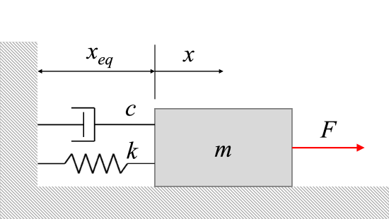
Consider the system above. The equation of the system becomes:
\[ m \ddot{x} + c \dot{x} + kx = F_0 \sin (\omega_0 t) \]
\[ \Rightarrow \ddot{x} + \frac{c}{m} \dot{x} + \frac{k}{m} x = \frac{F_0}{m} \ \sin (\omega_0 t). \]
Because the natural vibrations will damp out with friction (as mentioned in undamped harmonic vibrations), we will only consider the particular solution. This particular solution will have the form:
\[ x_p (t) = X' \sin (\omega_0 t - \phi '). \]
After solving, we determine that the expressions for \(X'\) and \(\phi '\) are:
\[ X' = \frac{ \dfrac{F_0}{k}}{ \sqrt{ \left[ 1 - \left( \dfrac{\omega_0}{\omega_n} \right) ^2 \right] ^2 + \left[ 2 \dfrac{c}{c_c} \dfrac{\omega_0}{\omega_n} \right] ^2 }} \]
\[ \phi ' = \tan ^{-1} \left[ \frac{ 2 \dfrac{c}{c_c} \dfrac{\omega_0}{\omega_n} }{1 - \left( \dfrac{\omega_0}{\omega_n} \right) ^2} \right]. \]
The magnification factor now becomes:
\[ MF = \frac{X'}{\dfrac{F_0}{k}} = \dfrac{1}{\sqrt{ \left[ 1 - \left( \dfrac{\omega_0}{\omega_n} \right) ^2 \right] ^2 + \left[ 2 \dfrac{c}{c_c} \dfrac{\omega_0}{\omega_n} \right] ^2 }} \]
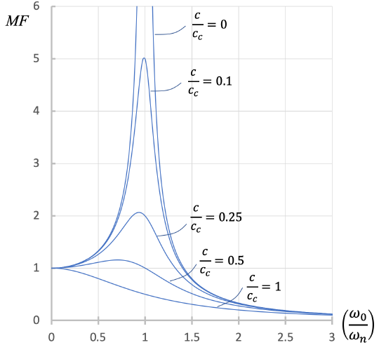
From the figure above, we can see that the extreme amplitudes at resonance only occur when the damping ratio = 0 and the ratio of frequencies is 1. Otherwise, damping inhibits the out-of-control vibrations that would otherwise be seen at resonance.
Worked Problems:
Question 1:
You are in a van that steadily accelerates from 20 m/s to 35 m/s over the course of 10 seconds. What is the rate of acceleration.

Solution:
Question 2:
You are in a van that steadily accelerates from 20 m/s to 35 m/s over the course of 10 seconds. How far did you travel in meters over the course of those ten seconds.

Solution:
Question 3:
A periodic force F=5sin(3t) is applied to a 5kg load, which is connected to a 10 N/m spring. Given that the floor’s coefficient of friction is μ=0.5, what is the maximum amplitude of the steady state function?

Solution:
Question 4:
A new fish species discovered in the Fraser River has been observed to be attracted to swinging pendulums as depicted above. You want to observe this phenomenon, so you take a spherical metal ball of mass m = 0.585 kg attached to a rope of length L = 1.5 m and tie it to a buoy as shown. If the drag force of the ball is modelled by Fd = −3v, what radius must the ball be for oscillation to occur? (Use g = 9.81 m/s2 and assume that sin θ = θ. Ignore the buoyancy force in your calculations.)

Solution:
Question 5:
Your latest invention is a milkshake maker that uses vibrational movement to create the perfect milkshake. You start by adding all the frozen ingredients to the milkshake maker and you can approximate it as a uniform, solid container. The milk shaker and all the ingredients inside have combined mass of m = 5.2 kg. It is connected to a damper with damping constant c = 8 N·s/m on one side, and a spring of stiffness k = 39 N/m on the other. A rotating wheel causes periodic motion to keep the milkshake shaking where δ0 = 41 cm and the angular velocity is ω = 4 rad/s. Find the damping ratio ζ, the phase angle φ′ of the steady state solution, the natural period of oscillation τn, the period of the steady state response τ0, and the period of the damped vibration τd.

Solution: