
15.4: Undamped Harmonic Forced Vibrations
- Page ID
- 50621

Often, mechanical systems are not undergoing free vibration, but are subject to some applied force that causes the system to vibrate. In this section, we will consider only harmonic (that is, sine and cosine) forces, but any changing force can produce vibration.
When we consider the free body diagram of the system, we now have an additional force to add: namely, the external harmonic excitation.
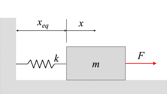
The equation of motion of the system above will be:
\[ m \ddot{x} + kx = F, \]
where \(F\) is a force of the form:
\[ F = F_0 \sin (\omega_0 t). \]
This equation of motion for the system can be re-written in standard form:
\[ \ddot{x} + \frac{k}{m} x = \frac{F_0}{m} \sin (\omega_0 t). \]
The solution to this system consists of the superposition of two solutions: a particular solution, \(x_p\) (related to the forcing function), and a complementary solution, \(x_c\) (which is the solution to the system without forcing).
As we saw previously, the complementary solution is the solution to the undamped free system: \[x_c = C \sin (\omega_n t + \phi). \]
We can obtain the particular solution by assuming a solution of the form: \[x_p = D \sin (\omega_0 t), \]
where \(\omega_0\) is the frequency of the harmonic forcing function. We differentiate this form of the solution, and then sub into the above equation of motion:
\[ \ddot{x}_p = - \omega_0^2 D \sin (\omega_0 t) \]
\[ - m \omega_0^2 D \sin (\omega_0 t) + k D \sin (\omega_0 t) = F_0 \sin (\omega_0 t) \]
After solving for \(D\), we can then use it to find the particular solution, \(x_p\):
\[ D = \frac{ \dfrac{F_0}{k}}{1 - \left( \dfrac{\omega_0}{\omega_n} \right) ^2} \]
\[ x_p = \frac{ \dfrac{F_0}{k}}{1 - \left( \dfrac{\omega_0}{\omega_n} \right) ^2} \ \sin (\omega_0 t). \]
Thus, the general solution for a forced, undamped system is:
\[ x_G (t) = \frac{ \dfrac{F_0}{k}}{1- \left( \dfrac{\omega_0}{\omega_n} \right) ^2} \ \sin (\omega_0 t) + C \sin (\omega_n t + \phi) \]
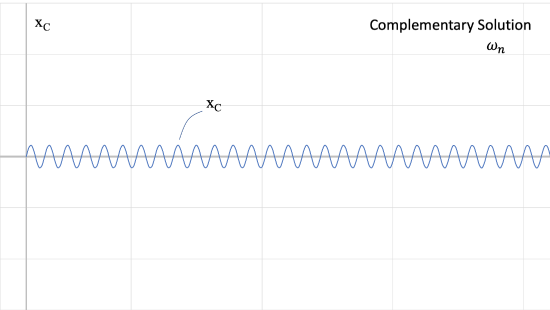
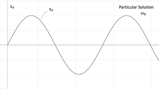
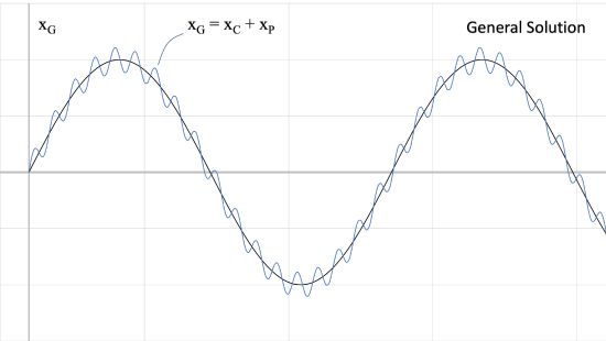
The above figures show the two responses at different frequencies. Recall that the value of \(\omega_n\) comes from the physical characteristics of the system (\(m, \, k\)) and \(\omega_0\) comes from the force being applied to the system. These responses are summed, to achieve the blue response (general solution) in Figure \(\PageIndex{4}\) above.
Steady-State Response:
In reality, this superimposed response does not last long. Every real system has some damping, and the natural response of the system will be damped out. As long as the external harmonic force is applied, however, the response to it will remain. When evaluating the response of the system to a harmonic forcing function, we will typically consider the steady-state response, when the natural response has been damped out and the response to the forcing function remains.
Amplitude of Forced Vibration
The amplitude of the steady-state forced vibration depends on the ratio of the forced frequency to the natural frequency. As \(\omega_0\) approaches \(\omega_n\) (the ratio approaches 1), the magnitude \(D\) becomes very large. We can define a magnification factor:
\[ MF = \dfrac{ \dfrac{ \dfrac{F_0}{k}}{1 - \left( \dfrac{\omega_0}{\omega_n} \right) ^2}} {\dfrac{F_0}{k}} = \dfrac{1}{1 - \left( \dfrac{\omega_0}{\omega_n} \right) ^2} \]
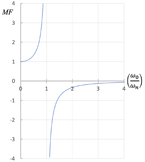
From the figure above, we can discuss various cases:
- \(\bf{\omega_0 = \omega_n}\): Resonance occurs. This results in very large-amplitude vibrations, and is associated with high stress and failure to the system.
- \(\bf{\omega_0 \sim 0, MF \sim 1}\): The forcing function is nearly static, leaving essentially the static deflection and limited natural vibration.
- \(\bf{\omega_0 < \omega_n}\): Magnification is positive and greater than 1, meaning the vibrations are in phase (when the force acts to the left, the system displaces to the left) and the amplitude of vibration is larger than the static deflection.
- \(\bf{\omega_0 > \omega_n}\): Magnification is negative and the absolute value is typically smaller than 1, meaning the vibration is out of phase with the motion of the forcing function (when the force acts to the left, the system displaces to the right) and the amplitude of vibration is smaller than the static deflection.
- \(\bf{\omega_0 >> \omega_n}\): The force is changing direction too fast for the block's motion to respond.
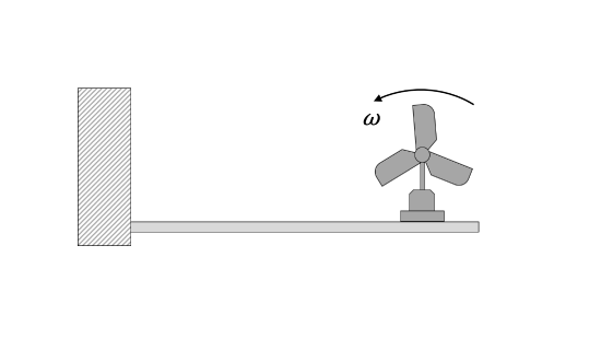
Rotating Unbalance:
One common cause of harmonic forced vibration in mechanical systems is rotating unbalance. This occurs when the axis of rotation does not pass through the center of mass, meaning that the center of mass experiences some acceleration instead of remaining stationary. This causes a force on the axle that changes direction as the center of mass rotates. We can represent this as a small mass, \(m\), rotating about the axis of rotation at some distance, called an eccentricity, \(e\). The forced angular frequency, \(\omega_0\), in this case is the angular frequency of the rotating system.
A 10-kg fan is fixed to a lightweight beam. The static weight of the fan deflects the beam by 20 mm. If the blade is designed to spin at \(\omega\) = 15 rad/s, and the blade is mounted off-center (equivalent to a 1.5 kg mass at 50 mm from the axis of rotation), determine the steady-state amplitude of vibration.
- Solution:
-
Video \(\PageIndex{1}\): Worked solution to example problem \(\PageIndex{1}\). YouTube source: https://youtu.be/k0vJLxaAjtw.
You are designing a stylish fan that uses only one blade. Approximate that blade as a narrow plate with a density per unit length of 20 g/cm. The base weight of the rest of the device (except for the blade) is 4 kg, and the whole thing is mounted on a lightweight beam. If the spring constant of the beam is \(k\) = 1000 N/m, find the length of blade than will cause resonance if the fan is designed to spin at \(\omega\) = 15 rad/s.

- Solution:
-
Video \(\PageIndex{2}\): Worked solution to example problem \(\PageIndex{2}\). YouTube source: https://youtu.be/tV4ETwwOyX0.