1.1: Introduction to Elastic Response

Introduction

This module outlines the basic mechanics of elastic response — a physical phenomenon that materials often (but do not always) exhibit. An elastic material is one that deforms immediately upon loading, maintains a constant deformation as long as the load is held constant, and returns immediately to its original undeformed shape when the load is removed. This module will also introduce two essential concepts in Mechanics of Materials: stress and strain.

Tensile strength and tensile stress

Perhaps the most natural test of a material’s mechanical properties is the tension test, in which a strip or cylinder of the material, having length L and cross-sectional area A, is anchored at one end and subjected to an axial load P – a load acting along the specimen’s long axis – at the other. (See Figure 1). As the load is increased gradually, the axial deflection δ of the loaded end will increase also. Eventually the test specimen breaks or does something else catastrophic, often fracturing suddenly into two or more pieces. (Materials can fail mechanically in many different ways; for instance, recall how blackboard chalk, a piece of fresh wood, and Silly Putty break.) As engineers, we naturally want to understand such matters as how δ is related to P, and what ultimate fracture load we might expect in a specimen of different size than the original one. As materials technologists, we wish to understand how these relationships are influenced by the constitution and microstructure of the material.

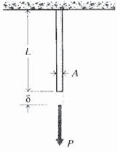
Figure 1: The tension test.

One of the pivotal historical developments in our understanding of material mechanical properties was the realization that the strength of a uniaxially loaded specimen is related to the magnitude of its cross-sectional area. This notion is reasonable when one considers the strength to arise from the number of chemical bonds connecting one cross section with the one adjacent to it as depicted in Figure 2, where each bond is visualized as a spring with a certain stiffness and strength. Obviously, the number of such bonds will increase proportionally with the section’s area(The surface density of bonds NS can be computed from the material’s density \(\rho\), atomic weight \(W_a\) and Avogadro’s number \(N_A\) as \(N_s = (\rho N_A/W_a)^{2/3}\). Illustrating for the case of iron (Fe):

\[N_S = \left(\dfrac{7.86 \tfrac{\text{g}}{\text{cm}^3} \cdot 6.023 \times 10^{23} \tfrac{\text{atoms}}{\text{mol}}}{55.85 \tfrac{\text{g}}{\text{mol}}}\right)^{\tfrac{2}{3}} = 1.9 \times 10^{15} \dfrac{\text{atoms}}{\text{cm}^2}\nonumber\]

\(N_S \approx 10^{15} \dfrac{\text{atom}}{\text{cm}^2}\) is true for many materials.). The axial strength of a piece of blackboard chalk will therefore increase as the square of its diameter. In contrast, increasing the length of the chalk will not make it stronger (in fact it will likely become weaker, since the longer specimen will be statistically more likely to contain a strength-reducing flaw.)

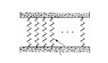
Figure 2: Interplanar bonds (surface density approximately \(10^{19}\ m^{-2}\)).

Galileo (1564–1642)(Galileo, Two New Sciences, English translation by H. Crew and A. de Salvio, The Macmillan Co., New York, 1933. Also see S.P. Timoshenko, History of Strength of Materials, McGraw-Hill, New York, 1953.) is said to have used this observation to note that giants, should they exist, would be very fragile creatures. Their strength would be greater than ours, since the cross-sectional areas of their skeletal and muscular systems would be larger by a factor related to the square of their height (denoted L in the famous DaVinci sketch shown in Figure 3). But their weight, and thus the loads they must sustain, would increase as their volume, that is by the cube of their height. A simple fall would probably do them great damage. Conversely, the “proportionate” strength of the famous arachnid mentioned weekly in the SpiderMan comic strip is mostly just this same size effect. There’s nothing magical about the muscular strength of insects, but the ratio of \(L^2\) to \(L^3\) works in their favor when strength per body weight is reckoned. This cautions us that simple scaling of a previously proven design is not a safe design procedure. A jumbo jet is not just a small plane scaled up; if this were done the load-bearing components would be too small in cross-sectional area to support the much greater loads they would be called upon to resist.

When reporting the strength of materials loaded in tension, it is customary to account for this effect of area by dividing the breaking load by the cross-sectional area:

\[\sigma_f = \dfrac{P_f}{A_0}\]

where \(\sigma_f\) is the ultimate tensile stress, often abbreviated as UTS, \(P_f\) is the load at fracture, and \(A_0\) is the original cross-sectional area. (Some materials exhibit substantial reductions in cross-sectional area as they are stretched, and using the original rather than final area gives the so-call engineering strength.) The units of stress are obviously load per unit area, \(N/m^2\) (also called Pascals, or Pa) in the SI system and \(lb/in^2\) (or psi) in units still used commonly in the United States.

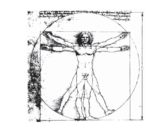
Figure 3: Strength scales with \(L^2\), but weight scales with \(L^3\).

Example \(\PageIndex{1}\)

In many design problems, the loads to be applied to the structure are known at the outset, and we wish to compute how much material will be needed to support them. As a very simple case, let’s say we wish to use a steel rod, circular in cross-sectional shape as shown in Figure 4, to support a load of 10,000 lb. What should the rod diameter be?

Figure 4: Steel rod supporting a 10,000 lb weight.

Directly from Equation 1.1.1, the area \(A_0\) that will be just on the verge of fracture at a given load \(P_f\) is

\[A_0 = \dfrac{P_f}{\sigma_f}\nonumber\]

All we need do is look up the value of \(\sigma_f\) for the material, and substitute it along with the value of 10,000 lb for \(P_f\), and the problem is solved.

A number of materials properties are listed in the Materials Properties module, where we find the UTS of carbon steel to be 1200 MPa. We also note that these properties vary widely for given materials depending on their composition and processing, so the 1200 MPa value is only a preliminary design estimate. In light of that uncertainty, and many other potential ones, it is common to include a “factor of safety” in the design. Selection of an appropriate factor is an often-difficult choice, especially in cases where weight or cost restrictions place a great penalty on using excess material. But in this case steel is relatively inexpensive and we don’t have any special weight limitations, so we’ll use a conservative 50% safety factor and assume the ultimate tensile strength is 1200/2 = 600 Mpa.

We now have only to adjust the units before solving for area. Engineers must be very comfortable with units conversions, especially given the mix of SI and older traditional units used today. Eventually, we’ll likely be ordering steel rod using inches rather than meters, so we’ll convert the MPa to psi rather than convert the pounds to Newtons. Also using \(A = \pi d^2/4\) to compute the diameter rather than the area, we have

\[d = \sqrt{\dfrac{4A}{\pi}} = \sqrt{\dfrac{4P_f}{\pi \sigma_f}} = \left[\dfrac{4 \times 10000 (lb)}{\pi \times 600 \times 10^6 (N/m^2) \times 1.449 \times 10^{-4} (\tfrac{lb/in^2}{N/m^2})}\right ]^{\tfrac{1}{2}} = 0.38\ in\nonumber\]

We probably wouldn’t order rod of exactly 0.38 in, as that would be an oddball size and thus too expensive. But \(3/8''\) (0.375 in) would likely be a standard size, and would be acceptable in light of our conservative safety factor.

If the specimen is loaded by an axial force \(P\) less than the breaking load \(P_f\), the tensile stress is defined by analogy with Equation 1.1.1 as

\[\sigma = \dfrac{P}{A_0}\]

The tensile stress, the force per unit area acting on a plane transverse to the applied load, is a fundamental measure of the internal forces within the material. Much of Mechanics of Materials is concerned with elaborating this concept to include higher orders of dimensionality, working out methods of determining the stress for various geometries and loading conditions, and predicting what the material’s response to the stress will be.

Example \(\PageIndex{2}\)

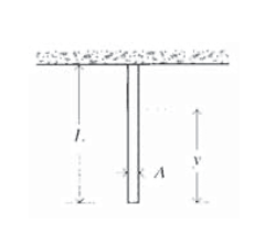
Figure 5: Circular rod suspended from the top and bearing its own weight.

Many engineering applications, notably aerospace vehicles, require materials that are both strong and lightweight. One measure of this combination of properties is provided by computing how long a rod of the material can be that when suspended from its top will break under its own weight (see Figure 5). Here the stress is not uniform along the rod: the material at the very top bears the weight of the entire rod, but that at the bottom carries no load at all.

To compute the stress as a function of position, let y denote the distance from the bottom of the rod and let the weight density of the material, for instance in \(N/m^3\), be denoted by \(\gamma\). (The weight density is related to the mass density \(\rho\) \([kg/m^3]\) by \(\gamma = \rho g\), where \(g = 9.8 m/s^2\) is the acceleration due to gravity.) The weight supported by the cross-section at \(y\) is just the weight density \(\gamma\) times the volume of material \(V\) below \(y\):

\[W(y) = \gamma V =\gamma Ay\nonumber\]

The tensile stress is then given as a function of \(y\) by Equation 1.1.2 as

\[\sigma(y) = \dfrac{W(y)}{A} = \gamma y\]

Note that the area cancels, leaving only the material density \(\gamma\) as a design variable.

The length of rod that is just on the verge of breaking under its own weight can now be found by letting \(y = L\) (the highest stress occurs at the top), setting \(\sigma (L) = \sigma_f\), and solving for \(L\):

\[\sigma_f = \gamma L \Rightarrow L = \dfrac{\sigma_f}{\gamma}\nonumber\]

In the case of steel, we find the mass density \(\rho\) in Appendix A to be \(7.85 \times 10^3 (kg/m^3)\); then

\[L = \dfrac{\sigma_f}{\rho g} = \dfrac{1200 \times 10^6 (N/m^2)}{7.85 \times 10^3 (kg/m^3) \times 9.8 (m/s^2)} = 15.6\ km\nonumber\]

This would be a long rod indeed; the purpose of such a calculation is not so much to design superlong rods as to provide a vivid way of comparing materials (see Exercise \(\PageIndex{4}\)).

Stiffness

It is important to distinguish stiffness, which is a measure of the load needed to induce a given deformation in the material, from the strength, which usually refers to the material’s resistance to failure by fracture or excessive deformation. The stiffness is usually measured by applying relatively small loads, well short of fracture, and measuring the resulting deformation. Since the deformations in most materials are very small for these loading conditions, the experimental problem is largely one of measuring small changes in length accurately.

Hooke(Robert Hooke (1635–1703) was a contemporary and rival of Isaac Newton. Hooke was a great pioneer in mechanics, but competing with Newton isn’t easy.) made a number of such measurements on long wires under various loads, and observed that to a good approximation the load \(P\) and its resulting deformation \(\delta\) were related linearly as long as the loads were sufficiently small. This relation, generally known as Hooke’s Law, can be written algebraically as

\[P = k\delta\]

where \(k\) is a constant of proportionality called the stiffness and having units of \(lb/in\) or \(N/m\). The stiffness as defined by \(k\) is not a function of the material alone, but is also influenced by the specimen shape. A wire gives much more deflection for a given load if coiled up like a watch spring, for instance.

A useful way to adjust the stiffness so as to be a purely materials property is to normalize the load by the cross-sectional area; i.e. to use the tensile stress rather than the load. Further, the deformation \(\delta\) can be normalized by noting that an applied load stretches all parts of the wire uniformly, so that a reasonable measure of “stretching” is the deformation per unit length:

\[\epsilon = \dfrac{\delta}{L_0}\]

Here \(L_0\) is the original length and \(\epsilon\) is a dimensionless measure of stretching called the strain. Using these more general measures of load per unit area and displacement per unit length(It was apparently the Swiss mathematician Jakob Bernoulli (1655-1705) who first realized the correctness of this form, published in the final paper of his life.), Hooke’s Law becomes:

\[\dfrac{P}{A_0} = E\dfrac{\delta}{L_0}\]

or

\[\sigma = E\epsilon\]

The constant of proportionality \(E\), called Young’s modulus(After the English physicist Thomas Young (1773–1829), who also made notable contributions to the under- standing of the interference of light as well as being a noted physician and Egyptologist.) or the modulus of elasticity, is one of the most important mechanical descriptors of a material. It has the same units as stress, Pa or psi. As shown in Figure 6, Hooke’s law can refer to either of Eqns. 1.1.3 or 1.1.6.

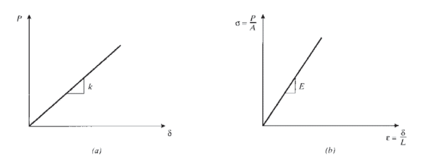
Figure 6: Hooke’s law in terms of (a) load-displacement and (b) stress-strain.

The Hookean stiffness \(k\) is now recognizable as being related to the Young’s modulus \(E\) and the specimen geometry as

\[k = \dfrac{AE}{L}\]

where here the 0 subscript is dropped from the area \(A\); it will be assumed from here on (unless stated otherwise) that the change in area during loading can be neglected. Another useful relation is obtained by solving Equation 1.1.5 for the deflection in terms of the applied load as

\[\delta = \dfrac{PL}{AE}\]

Note that the stress \(\sigma = P/A\) developed in a tensile specimen subjected to a fixed load is independent of the material properties, while the deflection depends on the material property \(E\). Hence the stress \(\sigma\) in a tensile specimen at a given load is the same whether it’s made of steel or polyethylene, but the strain \(\epsilon\) would be different: the polyethylene will exhibit much larger strain and deformation, since its modulus is two orders of magnitude less than steel’s.

Example \(\PageIndex{3}\)

In Example \(\PageIndex{1}\), we found that a steel rod \(0.38''\) in diameter would safely bear a load of 10,000 lb. Now let’s assume we have been given a second design goal, namely that the geometry requires that we use a rod 15 ft in length but that the loaded end cannot be allowed to deflect downward more than \(0.3''\) when the load is applied. Replacing \(A\) in Equation 1.1.8 by \(\pi d^2/4\) and solving for \(d\), the diameter for a given \(\delta\) is

\[d = 2 \sqrt{\dfrac{PL}{n\delta E}}\nonumber\]

From Appendix A, the modulus of carbon steel is 210 GPa; using this along with the given load, length, and deflection, the required diameter is

\[d = 2 \sqrt{\dfrac{10^4 (lb) \times 15 (ft) \times (in/ft)}{\pi \times 0.3 (in) \times 210 \times 10^9 (N/m^2) \times 1.449 \times 10^{-4} (\tfrac{lb/in^2}{N/m^2})}} = 0.5\ in \nonumber\]

This diameter is larger than the 0.38′′ computed earlier; therefore a larger rod must be used if the deflection as well as the strength goals are to be met. Clearly, using the larger rod makes the tensile stress in the material less and thus lowers the likelihood of fracture. This is an example of a stiffness- critical design, in which deflection rather than fracture is the governing constraint. As it happens, many structures throughout the modern era have been designed for stiffness rather than strength, and thus wound up being “overdesigned” with respect to fracture. This has undoubtedly lessened the incidence of fracture-related catastrophes, which will be addressed in the modules on fracture.

Example \(\PageIndex{4}\)

Figure 7: Deformation of a column under its own weight.

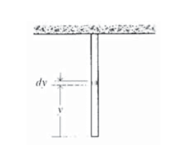
When very long columns are suspended from the top, as in a cable hanging down the hole of an oil well, the deflection due to the weight of the material itself can be important. The solution for the total deflection is a minor extension of Equation 1.1.8, in that now we must consider the increasing weight borne by each cross section as the distance from the bottom of the cable increases. As shown in Figure 7, the total elongation of a column of length \(L\), cross-sectional area \(A\), and weight density \(\gamma\) due to its own weight can be found by considering the incremental deformation \(d\delta\) of a slice dy a distance \(y\) from the bottom. The weight borne by this slice is \(\gamma Ay\), so

\[d \delta = \dfrac{(\gamma Ay) dy}{AE}\nonumber\]

\[\delta = \int_{0}^{L} \ d\delta = \dfrac{\gamma}{E} \dfrac{y^2}{2} |_{0}^{L} = \dfrac{\gamma L^2}{2E}\nonumber\]

Note that \(\delta\) is independent of the area \(A\), so that finding a fatter cable won’t help to reduce the deformation; the critical parameter is the specific modulus \(E/\gamma\). Since the total weight is \(W = \gamma AL\), the result can also be written

\[\delta = \dfrac{WL}{2AE}\nonumber\]

The deformation is the same as in a bar being pulled with a tensile force equal to half its weight; this is just the average force experienced by cross sections along the column.

In Example \(\PageIndex{2}\), we computed the length of a steel rod that would be just on the verge of breaking under its own weight if suspended from its top; we obtained \(L = 15.6\)km. Were such a rod to be constructed, our analysis predicts the deformation at the bottom would be

\[\delta = \dfrac{\gamma L^2}{2E} = \dfrac{7.85 \times 10^3 (kg/m^3) \times 9.8 (m/s^2) \times [15.6 \times 10^3 (m)]^2}{2 \times 210 times 10^9 (N/m^2)} = 44.6 \ m\nonumber\]

However, this analysis assumes Hooke’s law holds over the entire range of stresses from zero to fracture. This is not true for many materials, including carbon steel, and later modules will address materials response at high stresses.

A material that obeys Hooke’s Law (Equation 1.1.6) is called Hookean. Such a material is elastic according to the description of elasticity given in the introduction (immediate response, full recovery), and it is also linear in its relation between stress and strain (or equivalently, force and deformation). Therefore a Hookean material is linear elastic, and materials engineers use these descriptors interchangeably. It is important to keep in mind that not all elastic materials are linear (rubber is elastic but nonlinear), and not all linear materials are elastic (viscoelastic materials can be linear in the mathematical sense, but do not respond immediately and are thus not elastic).

The linear proportionality between stress and strain given by Hooke’s law is not nearly as general as, say, Einstein’s general theory of relativity, or even Newton’s law of gravitation. It’s really just an approximation that is observed to be reasonably valid for many materials as long the applied stresses are not too large. As the stresses are increased, eventually more complicated material response will be observed. Some of these effects will be outlined in the Module on Stress–Strain Curves, which introduces the experimental measurement of the strain response of materials over a range of stresses up to and including fracture.

If we were to push on the specimen rather than pulling on it, the loading would be described as compressive rather than tensile. In the range of relatively low loads, Hooke’s law holds for this case as well. By convention, compressive stresses and strains are negative, so the expression \(\sigma = E\epsilon\) holds for both tension and compression.

Exercise \(\PageIndex{1}\)

Determine the stress and total deformation of an aluminum wire, 30 m long and 5 mm in diameter, subjected to an axial load of 250 N.

Exercise \(\PageIndex{2}\)

Two rods, one of nylon and one of steel, are rigidly connected as shown. Determine the stresses and axial deformations when an axial load of \(F = 1\) kN is applied.

Exercise \(\PageIndex{3}\)

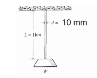
A steel cable 10 mm in diameter and 1 km long bears a load in addition to its own weight of \(W\) = 150 N. Find the total elongation of the cable.

Exercise \(\PageIndex{4}\)

Using the numerical values given in the Module on Material Properties,, rank the given materials in terms of the length of rod that will just barely support its own weight.

Exercise \(\PageIndex{5}\)

Plot the maximum self-supporting rod lengths of the materials in Exercise \(\PageIndex{4}\) versus the cost (per unit cross-sectional area) of the rod.

Exercise \(\PageIndex{6}\)

Show that the effective stiffnesses of two springs connected in (a) series and (b) parallel is

(a) series: \(\dfrac{1}{k_{eff}} = \dfrac{1}{k_1} + \dfrac{1}{k_2}\)

(b) parallel: \(k_{eff} = k_1 + k_2\)

(Note that these are the reverse of the relations for the effective electrical resistance of two resistors connected in series and parallel, which use the same symbols.)

Exercise \(\PageIndex{7}\)

A tapered column of modulus \(E\) and mass density \(\rho\) varies linearly from a radius of \(r_1\) to \(r_2\) in a length \(L\). Find the total deformation caused by an axial load \(P\).

Exercise \(\PageIndex{8}\)

A tapered column of modulus \(E\) and mass density \(\rho\) varies linearly from a radius of \(r_1\) to \(r_2\) in a length \(L\), and is hanging from its broad end. Find the total deformation due to the weight of the bar.

Exercise \(\PageIndex{9}\)

A rod of circular cross section hangs under the influence of its own weight, and also has an axial load \(P\) suspended from its free end. Determine the shape of the bar, i.e. the function \(r(y)\) such that the axial stress is constant along the bar’s length.

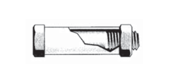
Exercise \(\PageIndex{10}\)

A bolt with 20 threads per inch passes through a sleeve, and a nut is threaded over the bolt as shown. The nut is then tightened one half turn beyond finger tightness; find the stresses in the bolt and the sleeve. All materials are steel, the cross-sectional area of the bolt is \(0.5 \ in^2\), and the area of the sleeve is \(0.4 \ in^2\).