3.2: Equilibrium

Introduction

The kinematic relations described in Module 8 are purely geometric, and do not involve considerations of material behavior. The equilibrium relations to be discussed in this module have this same independence from the material. They are simply Newton's law of motion, stating that in the absence of acceleration all of the forces acting on a body (or a piece of it) must balance. This allows us to state how the stress within a body, but evaluated just below the surface, is related to the external force applied to the surface. It also governs how the stress varies from position to position within the body.

Cauchy Stress

Figure 1: Traction vector.

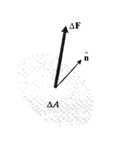
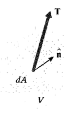
In earlier modules, we expressed the normal stress as force per unit area acting perpendicularly to a selected area, and a shear stress was a force per unit area acting transversely to the area. To generalize this concept, consider the situation depicted in Figure 1, in which a traction vector T acts on an arbitrary plane within or on the external boundary of the body, and at an arbitrary direction with respect to the orientation of the plane. The traction is a simple force vector having magnitude and direction, but its magnitude is expressed in terms of force per unit of area:

\[T = \lim_{\Delta A \to 0} \left (\dfrac{\Delta F}{\Delta A} \right )\]

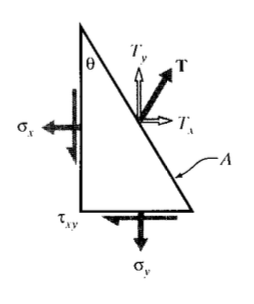
where \(\Delta A\) is the magnitude of the area on which ∆F acts. The Cauchy (Baron Augustin-Louis Cauchy (1789{1857) was a prolific French engineer and mathematician) stresses, which are a generalization of our earlier definitions of stress, are the forces per unit area acting on the Cartesian \(x\), \(y\), and \(z\) planes to balance the traction. In two dimensions this balance can be written by drawing a simple free body diagram with the traction vector acting on an area of arbitrary size \(A\) (Figure 2), remembering to obtain the forces by multiplying by the appropriate area.

\(\sigma_x (A \cos \theta) + \tau_{xy} (A \sin \theta) = T_x A\)

\(\tau_{xy} (A \cos \theta) + \sigma_{y} (A \sin \theta) = T_y A\)

Canceling the factor \(A\), this can be written in matrix form as

\[\begin{bmatrix} \sigma_x & \tau_{xy} \\ \tau_{xy} & \sigma_y \end{bmatrix} \left \{ \begin{array} {c} {\cos \theta} \\ {\sin \theta} \end{array} \right \} = \left \{ \begin{array} {c} {T_x} \\ {T_y} \end{array} \right \}\]

Figure 2: Cauchy stress.

Example \(\PageIndex{1}\)

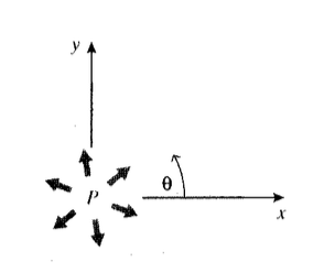
Consider a circular cavity containing an internal pressure \(p\). The components of the traction vector are then \(T_x = -p \cos \theta\), \(T_y = -p \sin \theta\). The Cartesian Cauchy stresses in the material at the boundary must then satisfy the relations

\(\sigma_x \cos \theta + \tau_{xy} \sin \theta = -p \cos \theta\)

\(\tau_{xy} \cos \theta + \sigma_y \sin \theta = -p \sin \theta\)

At \(\theta = 0, \sigma_x = -p, \sigma_y = \tau_{xy} = 0\); at \(\theta = \pi /2, \sigma_y = -p, \sigma_x = \tau_{xy} = 0\). The shear stress \(\tau_{xy}\) vanishes for \(\theta = 0\) or \(\pi /2\); in Module 10 it will be seen that the normal stresses \(\sigma_x\) and \(\sigma_y\) are therefore principal stresses at those points.

Figure 3: Constant pressure on internal circular boundary.

The vector \((\cos \theta, \sin \theta)\) on the left hand side of Equation 3.2.2 is also the vector \(\hat{n}\) of direction cosines of the normal to the plane on which the traction acts, and serves to define the orientation of this plane. This matrix equation, which is sometimes called Cauchy's relation, can be abbreviated as

\[[\sigma] \hat{n} = T\]

The brackets here serve as a reminder that the stress is being written as the square matrix of Equation 3.2.2 rather than in pseudovector form. This relation serves to define the stress concept as an entity that relates the traction (a vector) acting on an arbitrary surface to the orientation of the surface (another vector). The stress is therefore of a higher degree of abstraction than a vector, and is technically a second-rank tensor. The difference between vectors (first-rank tensors) and second-rank tensors shows up in how they transform with respect to coordinate rotations, which is treated in Module 10. As illustrated by the previous example, Cauchy's relation serves both to define the stress and to compute its magnitude at boundaries where the tractions are known.

Figure 4: Cartesian Cauchy stress components in three dimensions.

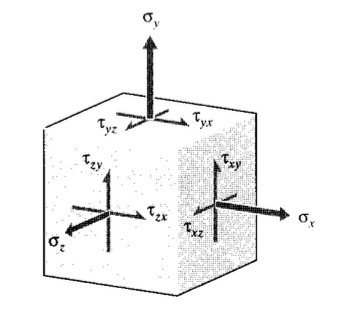
In three dimensions, the matrix form of the stress state shown in Figure 4 is the symmetric 3 \(\times\) 3 array obtained by an obvious extension of the one in Equation 3.2.2:

\[[\sigma] = \sigma_{i,j} = \begin{bmatrix} \sigma_x & \tau_{xy} & \tau_{xx} \\ \tau_{xy} & \sigma_y & \tau_{yx} \\ \tau_{xz} & \tau_{yz} & \sigma_z \end{bmatrix}\]

The element in the \(i^{\th}\) row and the \(j^{th}\) column of this matrix is the stress on the \(i^{th}\) face in the \(j^{th}\) direction. Moment equilibrium requires that the stress matrix be symmetric, so the order of subscripts of the off-diagonal shearing stresses is immaterial.

Differential Governing Equations

Determining the variation of the stress components as functions of position within the interior of a body is obviously a principal goal in stress analysis. This is a type of boundary value problem often encountered in the theory of differential equations, in which the gradients of the variables, rather than the explicit variables themselves, are specified. In the case of stress, the gradients are governed by conditions of static equilibrium: the stresses cannot change arbitrarily between two points \(A\) and \(B\), or the material between those two points may not be in equilibrium.

To develop this idea formally, we require that the integrated value of the surface traction T over the surface \(A\) of an arbitrary volume element \(dV\) within the material (see Figure 5) must sum to zero in order to maintain static equilibrium:

\(0 = \int_A T dA = \int_A [\sigma] \hat{n} dA\)

Here we assume the lack of gravitational, centripetal, or other "body" forces acting on material within the volume. The surface integral in this relation can be converted to a volume integral by Gauss' divergence theorem (Gauss' Theorem states that \(\int_A X \hat{n} dA = \int_S \nabla X dV\) where \(X\) is a scalar, vector, or tensor quantity.):

\(\int_V \nabla [\sigma] dV = 0\)

Since the volume \(V\) is arbitrary, this requires that the integrand be zero:

\[\nabla [\sigma] = 0\]

For Cartesian problems in three dimensions, this expands to:

\[\begin{array} {c} {\tfrac{\partial \sigma_x}{\partial x} + \tfrac{\partial \tau_{xy}}{\partial y} + \tfrac{\partial \tau_{xz}}{\partial z} = 0} \\ {\tfrac{\partial \tau_{xy}}{\partial x} + \tfrac{\partial \sigma_y}{\partial y} + \tfrac{\partial \tau_{yz}}{\partial z} = 0} \\ {\tfrac{\partial \tau_{xz}}{\partial x} + \tfrac{\partial \tau_{yz}}{\partial y} + \tfrac{\partial \sigma_z}{\partial x} = 0} \end{array}\]

Using index notation, these can be written:

\[\sigma_{ij, j} = 0\]

Or in pseudovector-matrix form, we can write

\[\begin{bmatrix} \tfrac{\partial}{\partial x} & 0 & 0 & 0 & \tfrac{\partial}{\partial z} & \tfrac{\partial}{\partial y} \\ 0 & \tfrac{\partial}{\partial y} & 0 & \tfrac{\partial}{\partial z} & 0 & \tfrac{\partial}{\partial x} \\ 0 & 0 & \tfrac{\partial}{\partial z} & \tfrac{\partial}{\partial y} & \tfrac{\partial}{\partial x} & 0 \end{bmatrix} \left \{ \begin{array} {c} {\sigma_x} \\ {\sigma_y} \\ {\sigma_z} \\ {\tau_{yz}} \\ {\tau_{xz}} \\ {\tau_{xy}} \end{array} \right \} = \left \{ \begin{array} {c} {0} \\ {0} \\ {0} \end{array} \right \}\]

Noting that the differential operator matrix in the brackets is just the transform of the one that appeared in Equation 3.2.7 of Module 8, we can write this as:

\[L^T \sigma = 0\]

Example \(\PageIndex{2}\)

It isn't hard to come up with functions of stress that satisfy the equilibrium equations; any constant will do, since the stress gradients will then be identically zero. The catch is that they must satisfy the boundary conditions as well, and this complicates things considerably. Later modules will outline several approaches to solving the equations directly, but in some simple cases a solution can be seen by inspection.

Figure 6: A tensile specimen.

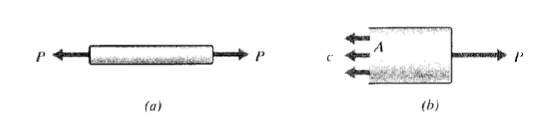
Consider a tensile specimen subjected to a load \(P\) as shown in Figure 6. A trial solution that certainly satisfies the equilibrium equations is

\[[\sigma] = \begin{bmatrix} c & 0 & 0 \\ 0 & 0 & 0 \\ 0 & 0 & 0 \end{bmatrix} \nonumber\]

where \(c\) is a constant we must choose so as to satisfy the boundary conditions. To maintain horizontal equilibrium in the free-body diagram of Figure 6(b), it is immediately obvious that \(cA = P\), or \(\sigma_x = c = P/A\). This familiar relation was used in Module 1 to define the stress, but we see here that it can be viewed as a consequence of equilibrium considerations rather than a basic definition.

Exercise \(\PageIndex{1}\)

Determine whether the following stress state satisfies equilibrium:

\([\sigma] = \begin{bmatrix} 2x^3y^2 & -2x^2y^3 \\ -2x^2y^3 & xy^4 \end{bmatrix}\)

Exercise \(\PageIndex{2}\)

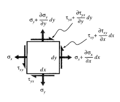
Develop the two-dimensional form of the Cartesian equilibrium equations by drawing a free-body diagram of an infinitesimal section:

Exercise \(\PageIndex{3}\)

Use the free body diagram of the previous problem to show that \(\tau_{xy} = \tau_{yx}\).

Exercise \(\PageIndex{4}\)

Use a free-body diagram approach to show that in polar coordinates the equilibrium equations are

\(\dfrac{\partial \tau_{r \theta}}{\partial r} + \dfrac{1}{r} \dfrac{\partial \sigma_{\theta}}{\partial \theta} + 2 \dfrac{\tau_{r \theta}}{r} = 0\)

Exercise \(\PageIndex{5}\)

Develop the above equations for equilibrium in polar coordinates by transforming the Cartesian equations using

\(x = r \cos \theta\)

\(y = r \sin \theta\)

Exercise \(\PageIndex{6}\)

The Airy stress function \(\phi (x, y)\) is defined such that the Cartesian Cauchy stresses are