
5.3: Solution for a Beam with Fixed Axial Displacements
- Page ID
- 21499
\( \newcommand{\vecs}[1]{\overset { \scriptstyle \rightharpoonup} {\mathbf{#1}} } \)
\( \newcommand{\vecd}[1]{\overset{-\!-\!\rightharpoonup}{\vphantom{a}\smash {#1}}} \)
\( \newcommand{\dsum}{\displaystyle\sum\limits} \)
\( \newcommand{\dint}{\displaystyle\int\limits} \)
\( \newcommand{\dlim}{\displaystyle\lim\limits} \)
\( \newcommand{\id}{\mathrm{id}}\) \( \newcommand{\Span}{\mathrm{span}}\)
( \newcommand{\kernel}{\mathrm{null}\,}\) \( \newcommand{\range}{\mathrm{range}\,}\)
\( \newcommand{\RealPart}{\mathrm{Re}}\) \( \newcommand{\ImaginaryPart}{\mathrm{Im}}\)
\( \newcommand{\Argument}{\mathrm{Arg}}\) \( \newcommand{\norm}[1]{\| #1 \|}\)
\( \newcommand{\inner}[2]{\langle #1, #2 \rangle}\)
\( \newcommand{\Span}{\mathrm{span}}\)
\( \newcommand{\id}{\mathrm{id}}\)
\( \newcommand{\Span}{\mathrm{span}}\)
\( \newcommand{\kernel}{\mathrm{null}\,}\)
\( \newcommand{\range}{\mathrm{range}\,}\)
\( \newcommand{\RealPart}{\mathrm{Re}}\)
\( \newcommand{\ImaginaryPart}{\mathrm{Im}}\)
\( \newcommand{\Argument}{\mathrm{Arg}}\)
\( \newcommand{\norm}[1]{\| #1 \|}\)
\( \newcommand{\inner}[2]{\langle #1, #2 \rangle}\)
\( \newcommand{\Span}{\mathrm{span}}\) \( \newcommand{\AA}{\unicode[.8,0]{x212B}}\)
\( \newcommand{\vectorA}[1]{\vec{#1}} % arrow\)
\( \newcommand{\vectorAt}[1]{\vec{\text{#1}}} % arrow\)
\( \newcommand{\vectorB}[1]{\overset { \scriptstyle \rightharpoonup} {\mathbf{#1}} } \)
\( \newcommand{\vectorC}[1]{\textbf{#1}} \)
\( \newcommand{\vectorD}[1]{\overrightarrow{#1}} \)
\( \newcommand{\vectorDt}[1]{\overrightarrow{\text{#1}}} \)
\( \newcommand{\vectE}[1]{\overset{-\!-\!\rightharpoonup}{\vphantom{a}\smash{\mathbf {#1}}}} \)
\( \newcommand{\vecs}[1]{\overset { \scriptstyle \rightharpoonup} {\mathbf{#1}} } \)
\(\newcommand{\longvect}{\overrightarrow}\)
\( \newcommand{\vecd}[1]{\overset{-\!-\!\rightharpoonup}{\vphantom{a}\smash {#1}}} \)
\(\newcommand{\avec}{\mathbf a}\) \(\newcommand{\bvec}{\mathbf b}\) \(\newcommand{\cvec}{\mathbf c}\) \(\newcommand{\dvec}{\mathbf d}\) \(\newcommand{\dtil}{\widetilde{\mathbf d}}\) \(\newcommand{\evec}{\mathbf e}\) \(\newcommand{\fvec}{\mathbf f}\) \(\newcommand{\nvec}{\mathbf n}\) \(\newcommand{\pvec}{\mathbf p}\) \(\newcommand{\qvec}{\mathbf q}\) \(\newcommand{\svec}{\mathbf s}\) \(\newcommand{\tvec}{\mathbf t}\) \(\newcommand{\uvec}{\mathbf u}\) \(\newcommand{\vvec}{\mathbf v}\) \(\newcommand{\wvec}{\mathbf w}\) \(\newcommand{\xvec}{\mathbf x}\) \(\newcommand{\yvec}{\mathbf y}\) \(\newcommand{\zvec}{\mathbf z}\) \(\newcommand{\rvec}{\mathbf r}\) \(\newcommand{\mvec}{\mathbf m}\) \(\newcommand{\zerovec}{\mathbf 0}\) \(\newcommand{\onevec}{\mathbf 1}\) \(\newcommand{\real}{\mathbb R}\) \(\newcommand{\twovec}[2]{\left[\begin{array}{r}#1 \\ #2 \end{array}\right]}\) \(\newcommand{\ctwovec}[2]{\left[\begin{array}{c}#1 \\ #2 \end{array}\right]}\) \(\newcommand{\threevec}[3]{\left[\begin{array}{r}#1 \\ #2 \\ #3 \end{array}\right]}\) \(\newcommand{\cthreevec}[3]{\left[\begin{array}{c}#1 \\ #2 \\ #3 \end{array}\right]}\) \(\newcommand{\fourvec}[4]{\left[\begin{array}{r}#1 \\ #2 \\ #3 \\ #4 \end{array}\right]}\) \(\newcommand{\cfourvec}[4]{\left[\begin{array}{c}#1 \\ #2 \\ #3 \\ #4 \end{array}\right]}\) \(\newcommand{\fivevec}[5]{\left[\begin{array}{r}#1 \\ #2 \\ #3 \\ #4 \\ #5 \\ \end{array}\right]}\) \(\newcommand{\cfivevec}[5]{\left[\begin{array}{c}#1 \\ #2 \\ #3 \\ #4 \\ #5 \\ \end{array}\right]}\) \(\newcommand{\mattwo}[4]{\left[\begin{array}{rr}#1 \amp #2 \\ #3 \amp #4 \\ \end{array}\right]}\) \(\newcommand{\laspan}[1]{\text{Span}\{#1\}}\) \(\newcommand{\bcal}{\cal B}\) \(\newcommand{\ccal}{\cal C}\) \(\newcommand{\scal}{\cal S}\) \(\newcommand{\wcal}{\cal W}\) \(\newcommand{\ecal}{\cal E}\) \(\newcommand{\coords}[2]{\left\{#1\right\}_{#2}}\) \(\newcommand{\gray}[1]{\color{gray}{#1}}\) \(\newcommand{\lgray}[1]{\color{lightgray}{#1}}\) \(\newcommand{\rank}{\operatorname{rank}}\) \(\newcommand{\row}{\text{Row}}\) \(\newcommand{\col}{\text{Col}}\) \(\renewcommand{\row}{\text{Row}}\) \(\newcommand{\nul}{\text{Nul}}\) \(\newcommand{\var}{\text{Var}}\) \(\newcommand{\corr}{\text{corr}}\) \(\newcommand{\len}[1]{\left|#1\right|}\) \(\newcommand{\bbar}{\overline{\bvec}}\) \(\newcommand{\bhat}{\widehat{\bvec}}\) \(\newcommand{\bperp}{\bvec^\perp}\) \(\newcommand{\xhat}{\widehat{\xvec}}\) \(\newcommand{\vhat}{\widehat{\vvec}}\) \(\newcommand{\uhat}{\widehat{\uvec}}\) \(\newcommand{\what}{\widehat{\wvec}}\) \(\newcommand{\Sighat}{\widehat{\Sigma}}\) \(\newcommand{\lt}{<}\) \(\newcommand{\gt}{>}\) \(\newcommand{\amp}{&}\) \(\definecolor{fillinmathshade}{gray}{0.9}\)The problem is solved under the assumption of simply-supported end condition, and the line load is distributed accordingly to the cosine function. The beam is restrained in the axial direction. There is a considerable strengthening effect of the beam response due to finite rotations of beam elements. The axial force \(N\) (non-zero this time) is calculated from Equation (5.1.6-5.1.7) with Equation (5.1.1)
\[N = EA \left[\frac{du}{dx} + \frac{1}{2}\left(\frac{dw}{dx}\right)^2\right] \label{6.15} \]
From Equation (5.1.4) we know that \(N\) is constant but unknown. In order to make use of the kinematic boundary conditions, let us integrate both sides of Equation \ref{6.15} with respect to \(x\)
\[\frac{Nl}{EA} = u(l) - u(0) + \int_{0}^{l} \frac{1}{2} \left( \frac{dw}{dx}\right)^2 dx\]
Using the boundary conditions for \(u\), the axial force is related to the square of the slope by
\[\frac{Nl}{EA} = \frac{1}{2} \int_{0}^{l} \left( \frac{dw}{dx}\right)^2 dx \label{6.17}\]
In order to determine the deflected shape of the beam, consider the equilibrium in the vertical direction given by Equation (5.1.5)
\[−EI \frac{d^4w}{dx^4} + N \frac{d^2w}{dx^2} + q = 0 \label{6.18}\]
Dividing both sides by \((−EI)\) one gets
\[\frac{d^4w}{dx^4} − \lambda^2 \frac{d^2w}{dx^2} = \frac{q_o}{EI} \cos \frac{\pi x}{l}\]
where
\[\lambda^2 = \frac{N}{EI}\]
The roots of the characteristic equations are \(0, 0, \pm \lambda\). Therefore the general solution of the homogeneous equation is
\[w_g = C_o + C_1x + C_2 \cosh \lambda x + C_3 \sinh \lambda x\]
As the particular solution of the inhomogeneous equation we can try
\[w_p(x) = C \cos \frac{\pi x}{l}\]
\[\frac{d^2w_p}{dx^2} = − \frac{\pi^2}{l^2} C \cos \frac{\pi x}{l}\]
\[\frac{d^4w_p}{dx^4} = \frac{\pi^4}{l^4} C \cos \frac{\pi x}{l}\]
Substituting the above solution to the governing equation \ref{6.18} one gets
\[\left[ \frac{\pi^4}{l^4} C - \lambda^2 \frac{\pi^2}{l^2} C - \frac{P_o}{EI} \right] \cos \frac{\pi x}{l} = 0\]
The above solution satisfy the differential equation if the amplitude \(C\) is related to input parameters and the unknown tension \(N\)
\[C = \frac{\frac{q_o}{EI}}{\frac{\pi^2}{l^2} \left(\lambda^2 + \frac{\pi^2}{l^2} \right)} = \frac{q_o}{EI \left(\frac{\pi}{l}\right)^4 + N\left(\frac{\pi}{l}\right)^2} \label{6.24}\]
The general solution of Equation \ref{6.18} is a sum of the particular solution of the inhomogeneous equation \(w_p\) and general solution of the homogeneous equation, \(w_g\)
\[w(x) = w_g + w_p \]
There are five unknowns, \(C_o, C_1, C_2, C_3\) and \(N\) and five equations. Four boundary conditions for the transverse deflections
\[w = 0, \quad \frac{d^2w}{dx^2} = 0 \quad \text{ at } \quad x = \pm \frac{l}{2}\]
and equation \ref{6.17} relating the horizontal and vertical response. The determination of the integration constants is straightforward. Note that the problem is symmetric. Therefore the solution should be an even function1 of \(x\). The terms \(C_1x\) and \(C_3 \sinh \lambda x are odd functions. Therefore the respective coefficients should vanish
\[C_1 = C_3 = 0 \]
\[w(x) = C_o + C_2 \cosh \lambda x + C \cos \frac{\pi x}{l} \label{6.28}\]
The remaining two coefficients are determined only from the boundary conditions at one side of the beam
\[\begin{array} w(x = \frac{l}{2} ) = 0 \rightarrow \\ \left. \frac{d^2w}{dx^2}\right|_{x = \frac{l}{2}} = 0 \rightarrow \end{array} \begin{cases} C_o + C_2 \cosh \frac{\lambda l}{2} = 0 \\ C_2\lambda^2 \cosh \frac{\lambda l}{2} = 0 \end{cases}\]
The solution of the above system is
\[C_o = C_2 = 0\]
The slope of the deflection curve, calculated from Equation \ref{6.28} is
\[\frac{dw}{dx} = −C \frac{\pi}{2} \sin \frac{\pi x}{2} \]
Expressing \(N\) in terms of \(x\) in Equation \ref{6.17} gives
\[\lambda^2 \left(\frac{Il}{A}\right) = \frac{1}{2} \int_{0}^{l} \left( \frac{dw}{dx}\right)^2 dx\]
Combining the above two equations one gets
\[\lambda^2 \left(\frac{Il}{A}\right) = \frac{1}{2} \int_{0}^{l} \left( - \frac{C\pi}{l} \sin \frac{\pi x}{l} \right)^2 dx\]
or after integration
\[\frac{\lambda^2 Il}{A} = \frac{1}{4} C^2 \left(\frac{\pi}{l} \right)^2 \frac{l}{2}\]
Recalling the definition of \(\lambda\), the membrane force \(N\) becomes a quadratic function of the deflection amplitude
\[N = \frac{EA}{4}C^2 \left(\frac{\pi}{l}\right)^2 \label{6.35}\]
The membrane force can be eliminated between Equations \ref{6.24} and \ref{6.35} to give the cubic equation for the deflection amplitude \(C\)
\[C + C^3 \frac{A}{4I} = \frac{q_o}{EI} \left(\frac{l}{\pi}\right)^4 \label{6.36}\]
To get a better sense of the contribution of various terms, consider a beam of the square cross-section \(h \times h\), for which
\[I = \frac{h}{12}, \; A = h^2, \; \frac{A}{I} = \frac{12}{h^2}\]
Also, the ventral deflection is dimensionalized with respect to the beam thickness \(\bar{w}_o = \frac{C}{h}\)
\[\bar{w}_o + 3w^{3}_o = \left(\frac{q_o}{Eh}\right) \left( \frac{l}{\pi h} \right)^4 \label{6.38}\]
The present solution is exact and involves all information about the material \((E)\), load intensity \((q_o)\), length \((l)\) and cross-sectional dimension. The distribution of line load and boundary conditions are reflected in the specific numerical coefficients in the respective terms.
In order to get a physical insight about the contributions of all terms in the above solution, consider two limiting cases:
- Pure bending solution for which \(N \frac{dw}{dx} = 0\).
- Pure membrane (string, cable) solution with zero flexural resistance (bending rigidity, \(EI \rightarrow 0\)).
(i) The bending solution is obtained by dropping the cubic term in Equations \ref{6.36} or \ref{6.38}
\[C = \frac{q_ol^4}{EI} \frac{1}{\pi^4} \label{6.39}\]
where the coefficient \(\pi^4 = 97.4\). this result for the sinusoidal distribution of the line load should be compared with the uniform line load (coefficient 77) and point load (coefficient 48).
(ii) The membrane solution is recovered by neglecting the first linear term
\[C^3 = \frac{q_ol^4}{EI} \frac{4}{\pi^4} \label{6.40}\]
The plot of the full bending/membrane solution and two limiting cases is shown in Figure (\(\PageIndex{1}\)).
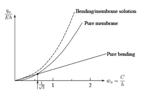
The question is at which magnitude of the central deflection relative to the beam thickness the non-dimensional load \(\frac{q_o}{Eh}\) is the same. This is the intersection of the straight line with the third order parabola. By eliminating the load parameter between Equations \ref{6.39} and \ref{6.40} one gets
\[C^2 = \frac{4I}{A} = \frac{4\rho^2 A}{A} = 4\rho^2\]
where \(\rho\) is the radius of gyration of the cross-section. For a square cross-section
\[C = 2\rho = 2\sqrt{\frac{I}{\rho}} = 2\sqrt{\frac{h^4}{12h^2}} = \frac{h}{\sqrt{3}} \cong 0.58h\]
It is concluded that the transition from bending to membrane action occurs quite early in the beam response. As a rule of thumb, the bending solution in the beam restrained from axial motion is restricted to deflections equal to half of the beam thickness. If deflections are larger, the membrane response dominate. For example, if beam deflection reaches three thicknesses, the contribution of bending and membrane action is 3:81. In the upper limit of the applicability of the theory of moderately large deflection of beams \(C \cong 10h\), the contribution of bending resistance is only 0.3% of the membrane strength.
The rapid transition from bending to membrane action is only present for axially restrained beams. If the beam is free to slide in the axial direction, no membrane resistance is developed and load is always linearly related to deflections.
The above elegant closed-form solution was obtained for the particular sinusoidal distribution of line load, which coincide with the deflected shape of the beam. For an arbitrary loading, only approximate solutions could be derived. One of such solution method, applicable to the broad class of non linear problems for plates and shells is called the Galerkin method.
1The function is even when \(f(−A) = f(A)\). The function is odd when \(f(−A) = −f(A)\).