2.1: Definition of a System

Last updated
Save as PDF

Page ID: 47226

Franz S. Hover & Michael S. Triantafyllou
Massachusetts Institute of Technology via MIT OpenCourseWare

\( \newcommand{\vecs}[1]{\overset { \scriptstyle \rightharpoonup} {\mathbf{#1}} } \) \( \newcommand{\vecd}[1]{\overset{-\!-\!\rightharpoonup}{\vphantom{a}\smash {#1}}} \)\(\newcommand{\id}{\mathrm{id}}\) \( \newcommand{\Span}{\mathrm{span}}\) \( \newcommand{\kernel}{\mathrm{null}\,}\) \( \newcommand{\range}{\mathrm{range}\,}\) \( \newcommand{\RealPart}{\mathrm{Re}}\) \( \newcommand{\ImaginaryPart}{\mathrm{Im}}\) \( \newcommand{\Argument}{\mathrm{Arg}}\) \( \newcommand{\norm}[1]{\| #1 \|}\) \( \newcommand{\inner}[2]{\langle #1, #2 \rangle}\) \( \newcommand{\Span}{\mathrm{span}}\) \(\newcommand{\id}{\mathrm{id}}\) \( \newcommand{\Span}{\mathrm{span}}\) \( \newcommand{\kernel}{\mathrm{null}\,}\) \( \newcommand{\range}{\mathrm{range}\,}\) \( \newcommand{\RealPart}{\mathrm{Re}}\) \( \newcommand{\ImaginaryPart}{\mathrm{Im}}\) \( \newcommand{\Argument}{\mathrm{Arg}}\) \( \newcommand{\norm}[1]{\| #1 \|}\) \( \newcommand{\inner}[2]{\langle #1, #2 \rangle}\) \( \newcommand{\Span}{\mathrm{span}}\)\(\newcommand{\AA}{\unicode[.8,0]{x212B}}\)

In short, a system is any process or entity that has one or more well-defined inputs and one or more well-defined outputs. Examples of systems include a simple physical object obeying Newtonian mechanics, and the US economy! Systems can be physical, or we may talk about a mathematical description of a system. The point of modeling is to capture in a mathematical representation the behavior of a physical system. As we will see, such representation lends itself to analysis and design, and certain restrictions such as linearity and time-invariance open a huge set of available tools.

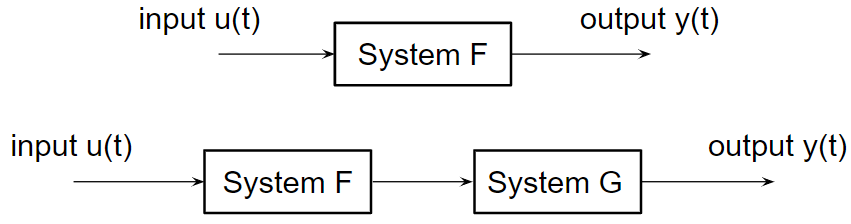
We often use a block diagram form to describe systems, and in particular their interconnections:

Sample of block diagram used to describe systems — Figure \(\PageIndex{1}\): Example of a simple block diagram used to describe two systems and their interconnection.

In the second case shown in Fig. 2.1.1, \(y(t) = G[F[u(t)]]\).

Looking at structure now and starting with the most abstracted and general case, we may write a system as a function relating the input to the output; as written these are both functions of time:

\[y(t) = F[u(t)] \nonumber\]

The system captured in \(F\) can be a multiplication by some constant factor - an example of a static system, or a hopelessly complex set of differential equations - an example of a dynamic system. If we are talking about a dynamical system, then by definition the mapping from \(u(t)\) to \(y(t)\) is such that the current value of the output \(y(t)\) depends on the past history of \(u(t)\). The following are several examples:

\[y(t) = \int\limits_{t-3}^{t} u^2(t_1)\, dt_1 \nonumber\]

\[y(t) = u(t) + \sum_{n=1}^N u(t - n \delta t) \nonumber\]

In the second case, \(\delta t\) is a a constant time step, and hence \(y(t)\) has embedded in it the current input plus a set of \(N\) delayed versions of the input.