2.2: Time-Invariant Systems

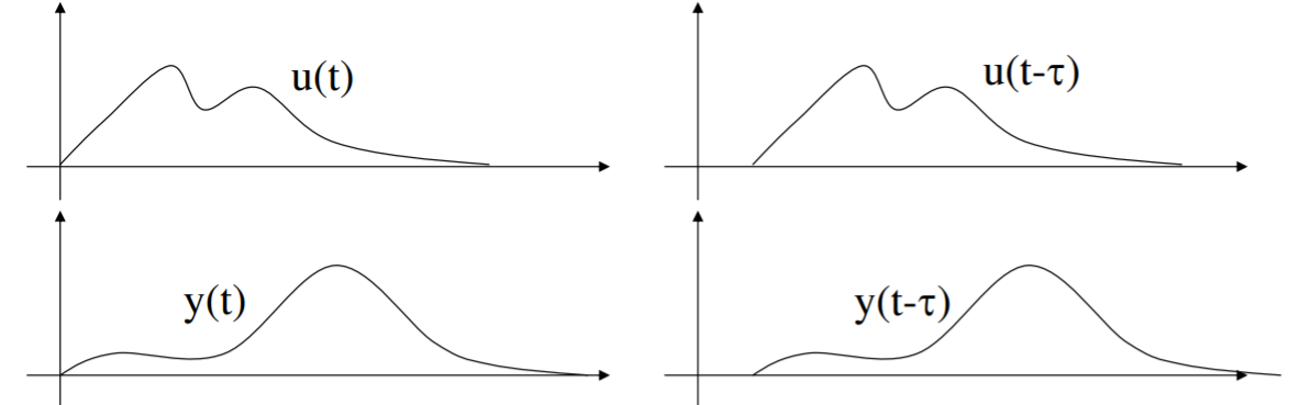
A dynamic system is time-invariant if shifting the input on the time axis leads to an equivalent shifting of the output along the time axis, with no other changes. In other words, a time-invariant system maps a given input trajectory \(u(t)\) no matter when it occurs:

\[y(t - \tau) = F[u(t - \tau)] \]

The formula above says specifically that if an input signal is delayed by some amount \(\tau\), so will be the output, and with no other changes.

Figure \(\PageIndex{1}\): Graphs of two physical time-invariant systems, \(u(t)\) and \(y(t)\). The shape of each graph does not change if the input signal is delayed by some amount \(\tau\), but is simply translated to the right by \(\tau\) units.

An example of a physical time-varying system is the pitch response of a rocket, \(y(t)\), when the thrusters are being steered by an angle \(u(t)\). You can see first that this is an inverted pendulum problem, and unstable without a closed-loop controller. It is time-varying because as the rocket burns fuel its mass is changing, and so the pitch responds differently to various inputs throughout its flight. In this case the ”absolute time” coordinate is the time since liftoff.

To assess whether a system is time-varying or not, follow these steps: replace \(u(t)\) with \(u(t − \tau)\) on one side of the equation, replace \(y(t)\) with \(y(t − \tau)\) on the other side of the equation, and then check if they are equal. Here are several examples.

\[y(t) = u(t)^{3/2}\]

This system is clearly time-invariant, because it is a static map. Next example:

\[y(t) = \int\limits_{0}^{t} \sqrt{u(t_1)}\, dt_1\]

Replace \(u(t_1)\) with \(u(t_1 - \tau)\) in the right-hand side and carry it through:

\[\int\limits_{0}^{t} \sqrt{u(t_1 - \tau)}\, dt_1 = \int\limits_{- \tau}^{t - \tau} \sqrt{u(t_2)}\, dt_2 \nonumber\]

The left-hand side is simply

\[y(t - \tau) = \int\limits_{0}^{t - \tau} \sqrt{u(t_1)}\, dt_1 \nonumber\]

Clearly the right- and left-hand sides are not equal (the limits of integration are different), and hence the system is not time-invariant. As another example, consider

\[y(t) = \int\limits_{t-5}^{t} u^2(t_1)\, dt_1 \]

The right-hand side becomes, with the time shift,

\[\int\limits_{t-5}^{t} u^2(t_1 - \tau)\, dt_1 = \int\limits_{t-5-\tau}^{t-\tau} u^2(t_2)\, dt_2 \nonumber \]

whereas the left-hand side is

\[y(t - \tau) = \int\limits_{t-5-\tau}^{t-\tau} u^2(t_1)\, dt_1 \nonumber \]

The two sides of the defining equation are equal under a time shift \(\tau\), and so this system is time-invariant. A subtlety here is encountered when considering inputs that are zero before time zero - this is the usual assumption in our work, namely \(u(t) = 0\) for \(t \leq 0\). While linearity is not affected by this condition, time invariance is, because the assumption is inconsistent with advancing a signal in time. Clearly part of the input would be truncated! Restricting our discussion to signal delays (the insertion of \(- \tau\) into the argument, where strictly \(\tau > 0\)) resolves the issue, and preserves time invariance as needed.