7.2: Single-Dimension Continuous Optimization

Consider the case of only one parameter, and one cost function. When the function is known and is continuous - as in many engineering applications - a very reasonable first method to try is to zero the derivative. In particular,

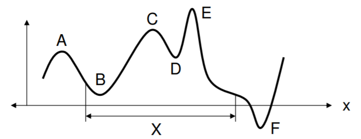
\[ \left[ \dfrac{df(x)}{dx} \right]_{x = x*} = 0. \] The user has to be aware even in this first problem that there can exist multiple points with a derivative of zero. These are any locations in \(X\) where \(f(x)\) is flat, and indeed these could be at local minima and at local and global maxima. Another important point to note is that if \(X\) is a finite domain, then there may be no location where the function is flat. In this case, the solution could lie along the boundary of \(X\), or take the minimum within \(X\). In the figure below, points \(A\) and \(C\) are local maxima, \(E\) is the global maxima, \(B\) and \(D\) are local minima, and \(F\) is the global minimum shown. However, the solution domain \(X\) does not admit \(F\), so the best solution would be \(B\). In all the cases shown, however, we have at the maxima and minima \(f'(x) = 0\). Furthermore, at maxima \(f''(x) < 0\), and at minima \(f''(x) > 0\).

Figure \(\PageIndex{1}\): graph of a sample function where points with zero derivative can easily be identified and parameter space \(X\) is taken into account, to identify points that maximize/minimize \(f(x)\) within the desired conditions.

We say that a function \(f(x)\) is convex if and only if it has everywhere a nonnegative second derivative, such as \(f(x) = x^2\). For a convex function, it should be evident that any minimum is in fact a global minimum. (A function is concave if \(-f(x)\) is convex.) Another important fact of convex functions is that the graph always lies above any points on a tangent line, defined by the slope at point of interest:

\[ f(x + \delta x) \geq f(x) + f'(x)\delta . \]

When \(\delta\) is near zero, the two sides are approximately equal.

Suppose that the derivative-zeroing value \(x^*\) cannot be deduced directly from the derivative. We need another way to move toward the minimum. Here is one approach: move in the downhill direction by a small amount that scales with the inverse of the derivative. Letting \(\delta = - \gamma / f'(x)\) makes the above equation:

\[ f(x + \delta) \approx f(x) - \gamma . \]

The idea is to take small steps downhill, e.g., \(x_{k+1} = x_k + \delta\) where \(k\) indicates the \(k\)'th guess, and this algorithm is usually just called a "gradient method" or something similarly nondescript! While it is robust, one difficulty with this algorithm is how to stop, because it tries to move a constant decrement in \(f\) at each step. It will be unable to do so near a flat minimum, although one can of course to modify \(\gamma\) on the fly to improve convergence.

As another method, propose a new problem in which \(g(x) = f'(x)\), and now we have to solve \(g(x^*)=0\). Finding the zero of a function is an important problem on its own. Now the convexity inequality above resembles the Taylor series expansion, which is rewritten here in full form:

\[ g(x + \delta) \, = \, g(x) + g'(x)\delta + \dfrac{1}{2!} g''(x) \delta^2 + \dfrac{1}{2!} g'''(x) \delta^3 + . \, . \, . \] The expansion is theoretically true for any \(x\) and any \(\delta\) (if the function is continuous), and so clearly \(g(x+\delta)\) can be at least approximated by the first two terms on the right-hand side. If it is desired to set \(g(x+\delta) = 0\), then we will have the estimate

\[ \delta = -g(x) / g'(x). \]

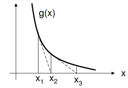
This is Newton’s first-order method for finding the zero of a function. The idea is to shoot down the tangent line to its own zero crossing, and take the new point as the next guess. As shown in the figure, the guesses could go wildly astray if the function is too flat near the zero crossing.

Figure \(\PageIndex{2}\): a error that must be considered when Newton's method is used to approximate the zero of a function; the lines tangent to the points \(x_1\) through \(x_3\) have progressively flatter slopes, and thus become increasingly likely to overshoot the zero of \(g(x)\) that is desired.

Let us view this another way. Going back to the function \(f\) and the Taylor series approximation

\[ f(x + \delta) \, \approx \, f(x) + f'(x)\delta + \dfrac{1}{2!}f''(x) \delta^2, \]

we can set to zero the left-hand side derivative with respect to \(\delta\), to obtain

\begin{align} 0 \, &\approx \, 0 + f'(x) + f''(x) \delta \longrightarrow \\[4pt] \delta \, &= \, -f'(x) / f''(x). \end{align}

This is the same as Newton’s method above since \(f'(x) = g(x)\). It clearly employs both first and second derivative information, and will hit the minimum in one shot(!) if the function truly is quadratic and the derivatives \(f'(x) and f''(x)\) are accurate. In the next section, which deals with multiple dimensions, we will develop an analogous and powerful form of this method. Also in the next section, we refer to a line search, which is merely a one-dimensional minimization along a particular direction, using a (unspecified) one-dimensional method ­- such as Newton’s method applied to the derivative.