7.8: Solving Dynamic Programming on a Computer

Last updated
Save as PDF

Page ID: 49285

Franz S. Hover & Michael S. Triantafyllou
Massachusetts Institute of Technology via MIT OpenCourseWare

\( \newcommand{\vecs}[1]{\overset { \scriptstyle \rightharpoonup} {\mathbf{#1}} } \) \( \newcommand{\vecd}[1]{\overset{-\!-\!\rightharpoonup}{\vphantom{a}\smash {#1}}} \)\(\newcommand{\id}{\mathrm{id}}\) \( \newcommand{\Span}{\mathrm{span}}\) \( \newcommand{\kernel}{\mathrm{null}\,}\) \( \newcommand{\range}{\mathrm{range}\,}\) \( \newcommand{\RealPart}{\mathrm{Re}}\) \( \newcommand{\ImaginaryPart}{\mathrm{Im}}\) \( \newcommand{\Argument}{\mathrm{Arg}}\) \( \newcommand{\norm}[1]{\| #1 \|}\) \( \newcommand{\inner}[2]{\langle #1, #2 \rangle}\) \( \newcommand{\Span}{\mathrm{span}}\) \(\newcommand{\id}{\mathrm{id}}\) \( \newcommand{\Span}{\mathrm{span}}\) \( \newcommand{\kernel}{\mathrm{null}\,}\) \( \newcommand{\range}{\mathrm{range}\,}\) \( \newcommand{\RealPart}{\mathrm{Re}}\) \( \newcommand{\ImaginaryPart}{\mathrm{Im}}\) \( \newcommand{\Argument}{\mathrm{Arg}}\) \( \newcommand{\norm}[1]{\| #1 \|}\) \( \newcommand{\inner}[2]{\langle #1, #2 \rangle}\) \( \newcommand{\Span}{\mathrm{span}}\)\(\newcommand{\AA}{\unicode[.8,0]{x212B}}\)

Certainly the above algorithm can be implemented as written - moving backward from the end to the beginning, keeping track at each stage only of the optimal trajectories from that stage forward. This decision will involve some careful recording and indexing. A very simple algorithm called value iteration may be more accessible on your first try. As we will show in an example below, value iteration also allows us to consider problems where distinct stages are not clear.

It goes this way:

Index all of the possible configurations, or nodes, of the system (cities).
With each configuration, create a list of where we can go to from that node - probably this is a list of indices (cities that are plausibly part of an optimal path). The starting node (Los Angeles) is pointed to by no other nodes, whereas the end node (Boston) points to none.
For each of these simple paths defined from node to node, assign a cost of transition (simple driving miles between the cities).
Now assign to each of these configurations an initial guess for the cost from this node to the end state (optimum total miles from each city to Boston). Clearly the costs-to-go for nodes that point to the terminal node are well-known, but none of the others are.
Sweep through all the configurations (except the terminal one), picking the best path out, based on the local path and the estimated cost at the next node. At each node, we have only to keep track of the best next node index, and the new estimated cost-to-go.
Repeat to convergence!

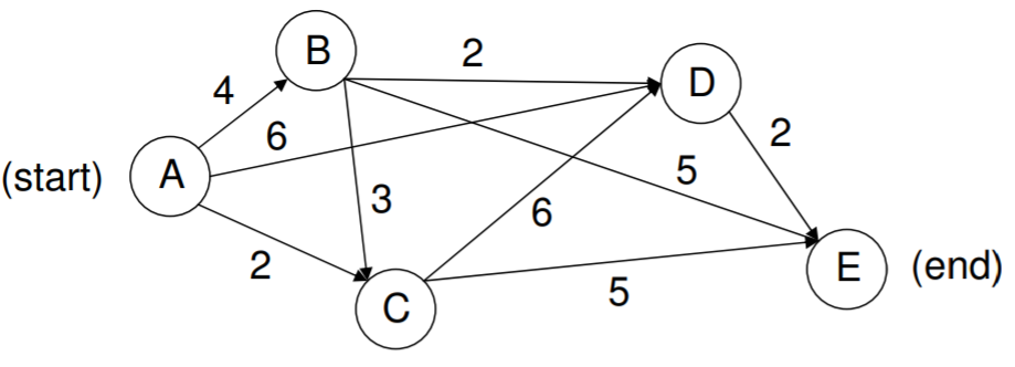
This algorithm can be shown to always converge, and has a number of variants and enhancements. An example makes things clearer:

Node	Points to Nodes	With Costs	Initial Estimate of Cost to Go
\(A\) (initial)	\(B, C, D\)	\(4, 2, 6\)	\(10\)
\(B\)	\(C, D, E\)	\(3, 2, 5\)	\(10\)
\(C\)	\(D, E\)	\(6, 5\)	\(10\)
\(D\)	\(E\)	\(2\)	\(2\) (known)
\(E\)	(terminal)	N/A	N/A

Visualization of a shortest-path problem with 3 nodes located at varying distances between a start and an end point. The costs of travel between any two nodes (the miles covered) are marked on the corresponding arrows. — Figure \(\PageIndex{1}\): locations of the five cities (nodes) are shown, along with the cost to travel from any one of the cities to any other in the direction that approaches the destination \(E\).

And here is the evolution of the value iteration:

Iteration	\(A\) cost-to-go	\(B\) cost-to-go	\(C\) cost-to-go	\(D\) cost-to-go
\(0\)	N/A	\(10\)	\(10\)	\(2(E)\)
\(1\)	\(\min (14, 12, 8) = 8(D, E)\)	\(\min (13, 4, 5) = 4(D, E)\)	\(\min (8, 5) = 5(E)\)	\(2(E)\)
\(2\)	\(\min (8, 7, 8) = 7(C, E)\)	\(4(D, E)\)	\(5(E)\)	\(2(E)\)

We can end safely after the second iteration because the path from \(A\) involves \(C\), which cannot change from its value after the first iteration, because it connects all the way through to \(E\).