11.4: Representing Linear Systems

The transfer function description of linear systems has already been described in the presentation of the Laplace transform. The state-space form is an entirely equivalent time-domain representation that makes a clean extension to systems with multiple inputs and multiple outputs, and opens the way to many standard tools from linear algebra.

Standard State-Space Form

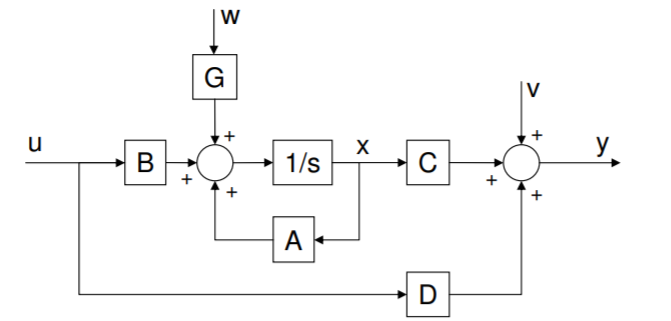
We write a linear system in a state-space form as follows

\begin{align} \dot{x} \,\, &= \,\, Ax + Bu + Gw \\[4pt] y \,\, &= \,\, Cx + Du + v \end{align}

where

• \(x\) is a state vector, with as many elements as there are orders in the governing differential equations.
• \(A\) is a matrix mapping \(x\) to its derivative; \(A\) captures the natural dynamics of the system without external inputs.
• \(B\) is an input gain matrix for the control input \(u\).
• \(G\) is a gain matrix for unknown disturbance \(w\); \(w\) drives the state just like the control \(u\).
• \(y\) is the observation vector, comprised mainly of a linear combination of states \(Cx\) (where \(C\) is a matrix).
• \(Du\) is a direct map from input to output (usually zero for physical systems).
• \(v\) is an unknown sensor noise which corrupts the measurement.

Figure \(\PageIndex{1}\): block diagram illustrates the relationship between the different variables introduced in Equations \(\PageIndex{1}\) - \(\PageIndex{2}\).

Converting a State-Space Model into a Transfer Function

Many different state-space descriptions can create the same transfer function - they are not unique. In the case of no disturbances or noise, the transfer function can be written as

\[ P(s) \, = \, \frac{y(s)}{u(s)} \, = \, C(sI - A)^{-1} B + D,\]

where \(I\) is the identity matrix with the same size as \(A\). To see that this is true, simply transform the differential equation into frequency space:

\begin{align*} sx(s) \,\, &= \,\, Ax(s) + Bu(s) \longrightarrow \\[4pt] x(s) (sI - A) \,\, &= \,\, Bu(s) \longrightarrow \\[4pt] x(s) \,\, &= \,\, (sI - A)^{-1} Bu(s) \longrightarrow \\[4pt] y(s) \,\, &= \,\, Cx(s) + Du(s) \,\, = \,\, C(sI - A)^{-1} Bu(s) + Du(s). \end{align*}

A similar equation holds for \(y(s)/w(s)\), and clearly \(y(s)/v(s) = 1\).

Converting a Transfer Function into a State-Space Model

Because state-space models are not unique, there are many different ways to create them from a transfer function. In the simplest case, it may be possible to write the corresponding differential equation along one row of the state vector, and then cascade derivatives. For example, consider the following system:

\begin{align*} my''(t) + by'(t) + ky(t) \,\, &= \,\, u'(t) + u(t) & \text{(mass-spring-dashpot)} \\[4pt] P(s) \,\, &= \,\, \frac{s+1}{ms^2 + bs + k} \end{align*}

Setting \(\vec{x} = [y', \, y]^T\), we obtain the system

\begin{align*} \dfrac{d \vec{x}}{dt} \,\, &= \,\, \begin{bmatrix} -b/m & -k/m \\[4pt] 1 & 0 \end{bmatrix} \vec{x} + \begin{bmatrix} 1/m \\[4pt] 0 \end{bmatrix} u \\[4pt] y \,\, &= \,\, [1 \quad 1] \vec{x} \end{align*}

Note specifically that \(dx_2 / dt = x_1\), leading to an entry of \(1\) in the off-diagonal of the second row in \(A\). Entries in the \(C\)-matrix are easy to write in this case because of linearity; the system response to \(u'\) is the same as the derivative of the system response to \(u\).