11.5: Block Diagrams and Transfer Functions of Feedback Systems

Block Diagrams: Fundamental Form

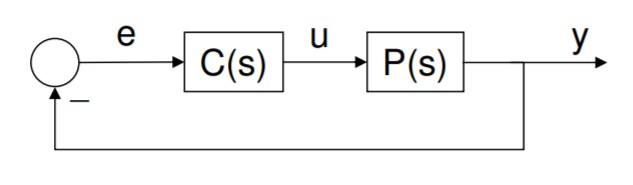
The topology of a feedback system can be represented graphically by considering each dynamical system element to reside within a box, having an input line and an output line. For example, a simple mass driven by a controlled force has transfer function \(P(s) = 1/ms^2\), which relates the input, force \(u(s)\), into the output, position \(y(s)\). In turn, the PD-controller (see below) has transfer function \(C(s) = k_p + k_d s\); its input is the error signal \(e(s) = -y(s)\), and its output force is \(u(s) = -(k_p + k_d s)y(s).\) This feedback loop in block diagram form is shown below.

Figure \(\PageIndex{1}\): block diagram of the feedback loop described above, showing the relationship between the inputs, outputs, and transfer functions.

Block Diagrams: General Case

The simple feedback system above is augmented in practice by three external inputs. The first is a process disturbance we call \(d\), which can be taken to act at the input of the physical plant, or at the output. In the former case, it is additive with the control action, and so has some physical meaning. In the second case, the disturbance has the same units as the plant output.

Another external input is the reference command or setpoint, used to create a more general error signal \(e(s) = r(s)-y(s).\) Note that the feedback loop, in trying to force \(e(s)\) to zero, will necessarily make \(y(s)\) approximate \(r(s).\)

The final input is sensor noise \(n\), which usually corrupts the feedback signal \(y(s)\), causing some error in the evaluation of \(e(s)\), and so on. Sensors with very poor noise properties can ruin the performance of a control system, no matter how perfectly understood are the other components.

Note that the disturbances \(d_u\) and \(d_y\), and the noise \(n\) are generalizations on the unknown disturbance and sensor noise we discussed at the beginning of this section.

Figure \(\PageIndex{1}\), accounting for the additional factors of process disturbance \(d\), reference command \(r\), and sensor noise \(n\).

Transfer Functions

Some algebra applied to the above figure (and neglecting the Laplace variable \(s\)) shows that

\begin{align} \frac{e}{r} \,\, &= \,\, \frac{1}{1 + PC} \,\, = \,\, S \\[4pt] \frac{y}{r} \,\, &= \,\, \frac{PC}{1 + PC} \,\, = \,\, T \\[4pt] \frac{u}{r} \,\, &= \,\, \frac{C}{1 + CP} \,\, = \,\, U. \end{align}

Let us derive the first of these. Working directly from the figure, we have

\begin{align*} e(s) \,\, &= \,\, r(s) - y(s) \\[4pt] e(s) \,\, &= \,\, r(s) - P(s) u(s) \\[4pt] e(s) \,\, &= \,\, r(s) - P(s) C(s) e(s) \\[4pt] (1 + P(s)C(s)) e(s) \,\, &= \,\, r(s) \\[4pt] \frac{e(s)}{r(s)} \,\, &= \,\, \frac{1}{1 + P(s)C(s)}. \end{align*}

The fact that we are able to make this kind of construction is a direct consequence of the frequency-domain representation of the system, and namely that we can freely multiply and divide system impulse responses and signals, so as to represent convolutions in the time-domain.

Now \(e/r = S\) relates the reference input and noise to the error, and is known as the sensitivity function. We would generally like \(S\) to be small at certain frequencies, so that the non-dimensional tracking error \(e/r\) there is small. \(y/r = T\) is called the complementary sensitivity function. Note that \(S+T = 1\), implying that these two functions must always trade off; they cannot both be small or large at the same time. Other systems we encounter again later are the (forward) loop transfer function \(PC\); the loop transfer function broken between \(C\) and \(P\), namely \(CP\); and some others:

\begin{align} \frac{e}{d_u} \,\, &= \,\, \frac{-P}{1 + PC} \\[4pt][4 pt] \frac{y}{d_u} \,\, &= \,\, \frac{P}{1 + PC} \\[4pt][4 pt] \frac{u}{d_u} \,\, &= \,\, \frac{-CP}{1 + CP} \\[4pt][4 pt] \frac{e}{d_y} \,\, &= \,\, \frac{-1}{1 + PC} \,\, = \,\, -S \\[4pt][4 pt] \frac{y}{d_y} \,\, &= \,\, \frac{1}{1 + PC} \,\, = \,\, S \\[4pt][4 pt] \frac{u}{d_y} \,\, &= \,\, \frac{-C}{1 + CP} \,\, = \,\, -U \\[4pt][4 pt] \frac{e}{n} \,\, &= \,\, \frac{-1}{1 + PC} \,\, = \,\, -S \\[4pt][4 pt] \frac{y}{n} \,\, &= \,\, \frac{-PC}{1 + PC} \,\, = \,\, -T \\[4pt][4 pt] \frac{u}{n} \,\, &= \,\, \frac{-C}{1 + CP} \,\, = \,\, -U. \end{align}

If the disturbance is taken at the plant output, then the three functions \(S\), \(T\), and \(U\) (control action) completely describe the system. This will be the procedure when we address loopshaping.