Chapter 6: Mechanical Behavior of Materials Part II

6.1 Linear Viscoelasticity (LVE):

I have recorded a series of lectures videos to supplement this text which can be found in the playlist below:

https://www.youtube.com/playlist?lis...b5i6HX2SGPPNyA

So far we have dealt with continuum isotropic linear elasticity and anisotropic linear elasticity. All these modes of deformation are independent of time, rate, and temperature. However, today we will discuss linear viscoelasticity whose deformation is governed by time, rate, and temperature. Linear viscoelasticity is the deformation between that of an elastic solid and a viscous fluid. We can actually see this in the name linear viscoelasticity. There is still a linear relationship between stress and strain for a given time and temperature. The visco term denotes a time component and elasticity denotes reversibility. The elastic solid will again behave Hookean with the relationship

\begin{equation}
\sigma = E \epsilon
\end{equation}

and the viscous fluid will be governed by this new equation

\begin{equation}
\sigma = \eta \dot{\epsilon}
\end{equation}

Linear Viscoelasticity is typically used to describe the mechanical response for polymers, glasses, tissues, and cells.

When a viscous fluid is deformed under an applied shear stress there is no recovery when the shear stress is removed so our equation for shear stress becomes

\begin{equation}
\tau = \eta \dot{\gamma}
\end{equation}

where \(\eta\) is the fluid viscosity (units of Pa s) and \(\dot{\gamma}\) is the shear strain rate (units of inverse seconds). Again this is linear because there is a proportional increase in \(\sigma\) and \(\epsilon\) for some time or temperature.

We can make a couple of linear viscoelastic (LVE) models which describe some LVE behavior phenomonolgically as combinations of springs and dashpots.

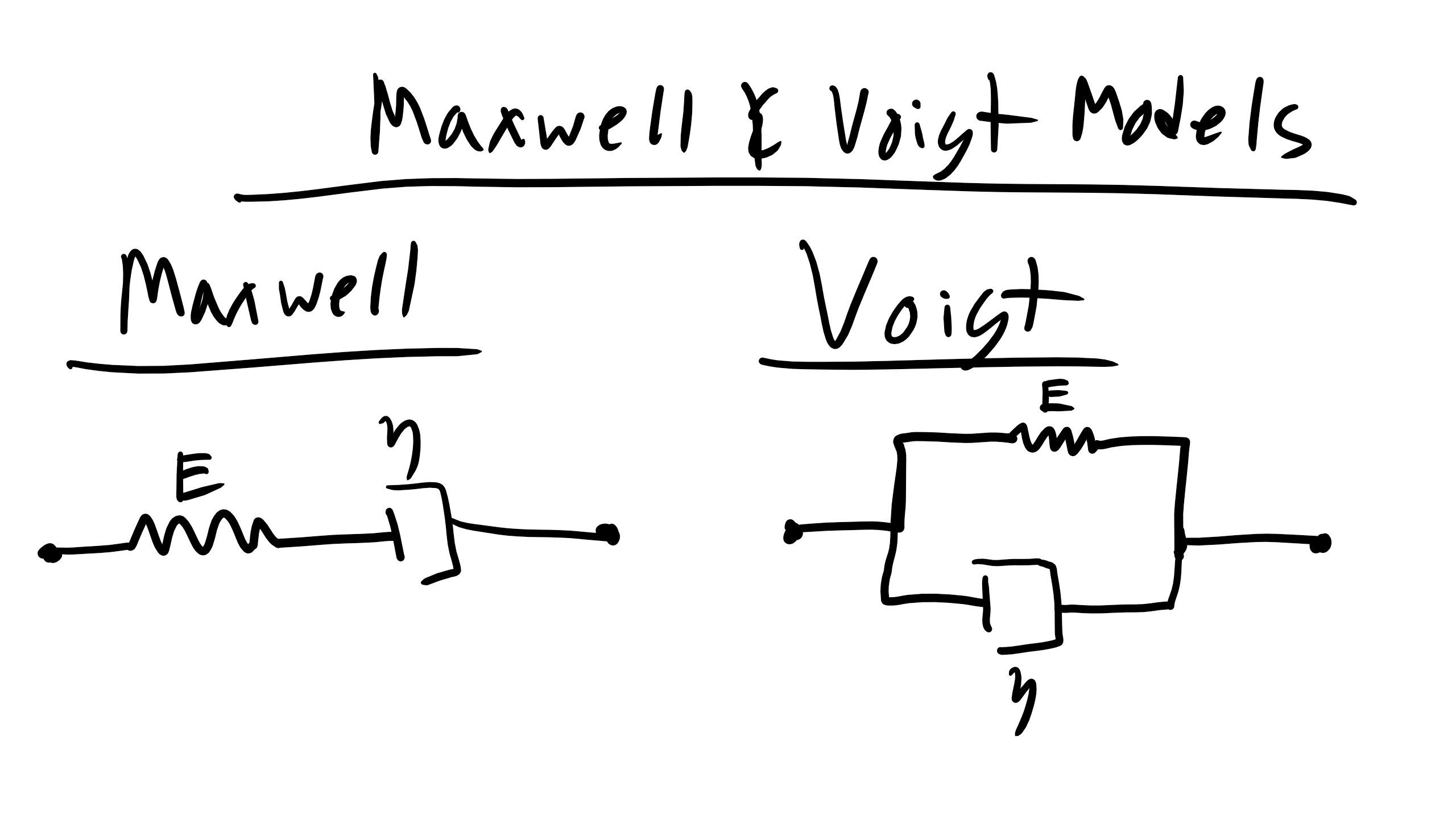
Maxwell Model:

Let’s take a look at the Maxwell model which is a combination of a spring in series with a dashpot that contains a Newtonian fluid.

The spring is described by the following equation:

\begin{equation}
\sigma_{s} = E_{s}\epsilon_{s}
\end{equation}

where \(\sigma_s\) is the stress in the spring, \(E_s\) is the stiffness of the spring, and \(\epsilon_s\) is the strain in the spring

The dashpot is described by:

\begin{equation}
\sigma_{d} = \eta_{d} \dot{\epsilon_{d}}
\end{equation}

where \(\sigma_d\) is the stress in the dashpot, \(\eta_d\) is the viscosity of the dashpot, and \(\dot{\epsilon_{d}}\) is the strain rate of the dashpot.

Now let’s say that I stress the system (this should be reminiscent of the composites pulled transverse to the fiber direction when we get to this) the stresses should be the same for the spring and the dashpot however the strains in the dashpot and the spring will be different which gives us the following equation:

\begin{eqnarray}
\sigma_{M} = \sigma_{s}=\sigma_{d}\\
\epsilon_{M} = \epsilon_{s} + \epsilon_{d}\\
\dot{\epsilon_{M}} = \dot{\epsilon_{s}} + \dot{\epsilon_{d}}\\
\dot{\epsilon_{M}} = \frac{\dot{\sigma_{M}}}{E} + \frac{\sigma_{M}}{\eta}
\end{eqnarray

With this system we can do two types of experiments: stress relaxation ( \(\epsilon = \epsilon_0\) i.e. constant strain) and creep (\(\sigma= \sigma_0\), i.e. constant stress).

For stress relaxation we can plug into our equation and solve for how the stress in our Maxwell model should vary over time:

\begin{eqnarray}
0=\frac{1}{E}\frac{d\sigma}{dt}+\frac{\sigma}{\eta}\\
\int^{\sigma}_{\sigma_{0}}\frac{d\sigma}{\sigma} = \int^{t}_{0}\frac{-E}{\eta}dt\\
\sigma(t) =\sigma_{0}\exp\bigg(\frac{-Et}{\eta}\bigg)\\
\sigma(t) =\sigma_{0}\exp\bigg(\frac{-t}{\tau}\bigg)
\end{eqnarray}

where \(\tau = \frac{E}{\eta}\) is the relaxation time. Similarly for creep:

\begin{eqnarray}
\frac{d\epsilon}{dt} = 0 + \frac{\sigma_{0}}{\eta}\\
\int^{\epsilon}_{\epsilon_{0}}d\epsilon = \int^{t}_{0}\frac{\sigma_{0}}{\eta}dt\\
\epsilon(t) = \epsilon_{0} + \frac{\sigma_{0}t}{\eta}
\end{eqnarray}

Kelvin-Voigt Model:

There is also the Kelvin-Voigt (KV) model has the spring and dashpot series in parallel.

In this case now the strain is the same but now the stresses are different so we get:

\begin{eqnarray}
\epsilon_{KV} = \epsilon_{s} = \epsilon_{d}\\
\sigma_{KV} = \sigma_{s} + \sigma_{d}\\
\sigma_{KV} = E_{s}\epsilon_{s}+\eta_{d}\dot{\epsilon_{d}}\\
\dot{\epsilon_{KV}} = \frac{\sigma_{KV}}{\eta_{d}} - \frac{E_{s}}{\eta_{d}}\epsilon_{KV}
\end{eqnarray}

Now for stress relaxation we get the final equation for stress vs time as:

\begin{equation}
\sigma(t) = E\epsilon_{0}
\end{equation}

and for creep we get:

\begin{equation}
\epsilon(t) = \frac{\sigma_{0}}{E}\bigg(1-\exp[-\frac{t}{\tau}]\bigg)
\end{equation}

You can now build even more complex combinations to model viscoelastic properties like the Standard Linear Viscoelastic Solid Model. Perhaps a more useful experimental measurement for visoelastic behavior is accomplished by Dynamic Mechanical Testing.

6.2 Dynamic Mechanical Testing:

The more utilized characterization technique is typically some type of dynamic mechanical testing to probe the viscoelastic behavior of materials. In this experiment the polymer is subjected of a sinusoidal loading at variable frequencies which can be described as such as
\begin{equation}
\sigma_{applied} = \sigma_o \sin \omega t
\end{equation}

This is the applied stress but remember we are dealing with a viscoelastic material so there will be a phase lag, \(\delta\), in the strain behavior which will also be sinusoidal

\begin{equation}
\epsilon = \epsilon_o \sin \omega t
\end{equation}

So what we will end up with is that the material will actually experience a stress that contains the phase lag as shown below

\begin{eqnarray}
\sigma = \sigma_o \sin (\omega t + \delta)\\
\sigma = \sigma_o \sin \omega t \cos \delta + \sigma_o \cos \omega t \sin \delta
\end{eqnarray}

where in the equation above we just expanded our trig functions. Notice here that the first term represents the component that is in phase with the strain or the elastic response while the second term represents the out of phase behavior or the viscous response. We can then define two elastic moduli to describe the in-phase and out of phase behavior. The storage or elastic modulus is the in-phase contribution and defined as

\begin{equation}
E' = \frac{\sigma_o \cos \delta}{\epsilon_o}
\end{equation}

and the loss modulus is the out of phase component is

\begin{equation}
E'' = \frac{\sigma_o \sin \delta }{\epsilon_o}
\end{equation}

We can now re-write our expression for the stress in the material as

\begin{equation}
\sigma = E' \sin \omega t + E'' \cos \omega t
\end{equation}

then by definition we have that

\begin{equation}
\tan \delta = \frac{E''}{E'}
\end{equation}

This is sometimes called the loss tangent and essentially represents the amount of energy lost over the energy stored[9]. You might also see these expressions written using complex variables like so

\begin{eqnarray}
\epsilon = \epsilon_o \exp i \omega t\\
\sigma = \sigma \exp i\omega t + \delta\\
E = \frac{\sigma_o}{\epsilon_o} \exp i \delta = \frac{\sigma_o}{\epsilon_o} (\cos \delta + i \sin \delta) = E' + E''
\end{eqnarray}

Analysis of DMA Experiments:

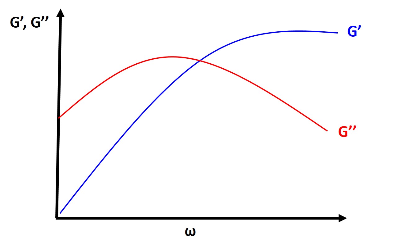
Typically you will find, at a fixed temperature that the loss tangent and the loss modulus are typically very small at very low and and very high frequencies and they will typically peak at intermediate frequencies. The storage modulus is high at high frequencies (short times) which should make sense intuitively as polymers will typically behave glassy or elastic at high frequencies and short times (strain rate is faster than relaxation time of polymer) and at low frequencies (long time longer than relaxation time) the polymer will behave more like a vicious fluid.

More importantly from this analysis we can determine experimentally the characteristic relaxation time from the point where \(G^'\) and \(G^''\) intersect. More often we will find that typical DMA experiments where \(G^'\), \(G^''\), and \(\tan \delta\) are plotted as a function of temperature. Here you will typically see larger peaks and changes in these parameters. The amount of molecular motion and free volume will increase and this will affect these properties, particularly the loss tangent. So you will expect to see large changes at the glass transition temperature and melting temperature but you also might expect to see other small peaks associated with secondary transitions (note this is not referring to second order thermodynamic transitions like \(T_g\) this is just referring to the magnitude of the peaks) associated with molecular motion of the polymer such as the temperature at which backbone side group rotation is accessible.

6.3 Composite Mechanics:

So far we have been talking about the mechanics of primarily metals but we haven’t really touched on composite mechanics. Composites materials are materials that contain typically more than one type of material combined. This typically involves a material matrix which is the major component in terms of volume fraction. This matrix material is reinforced by an additional material typically one that is stiffer or tougher than matrix material. The material that reinforces the matrix can be in particle form, fibers, or precipitates. A composite can also be a porous material like metal foams, concrete, ECM, etc.

Let’s take a look at a particle reinforced composite that is composed of a matrix which has some elastic modulus, \(E_m\), and volume fraction, \(f_m\). There is also the particle reinforcement in this case which again has an associated elastic modulus, \(E_p\), and volume fraction \(f_p\). Thus the total composite modulus, \(E_{composite}\) is

\begin{equation}
E_{composite} = E_{m}f_{m} + E_{p}f_{p}
\end{equation}

empirically there is typically a constant that is less than 1 for the particle reinforcement contribution but again that constant can only be found empirically.

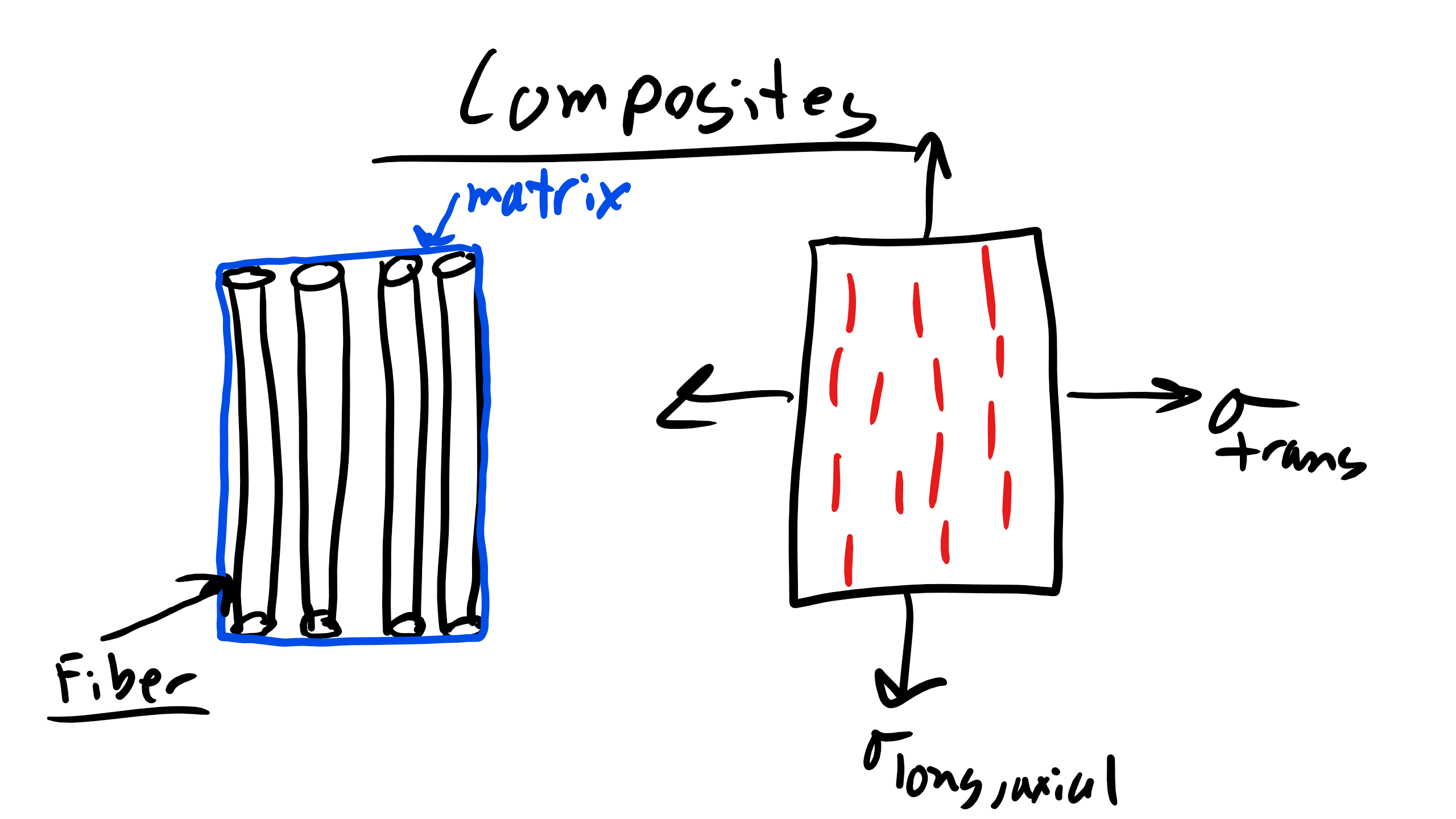
Let’s now look at a fiber reinforced composite that is pulled or stressed in the transverse direction with respect the the longitudinal or axial direction of the fibers. The stresses are the same on the matrix and the fibers. However the strains of the fiber and matrix will be different. With these constraints:

\begin{eqnarray}
\sigma_{m}=\sigma_{f}=\sigma\\
\epsilon_{c} = \epsilon_{m}f_{m} + \epsilon_{f}f_{f} \\
\epsilon_{c} = \sigma\bigg(\frac{f_{m}}{E_{m}} + \frac{f_{f}}{E_{f}}\bigg)\\
\frac{1}{E_{c}} = \frac{f_{f}}{E_{f}} + \frac{f_{m}}{E_{m}}
\end{eqnarray}

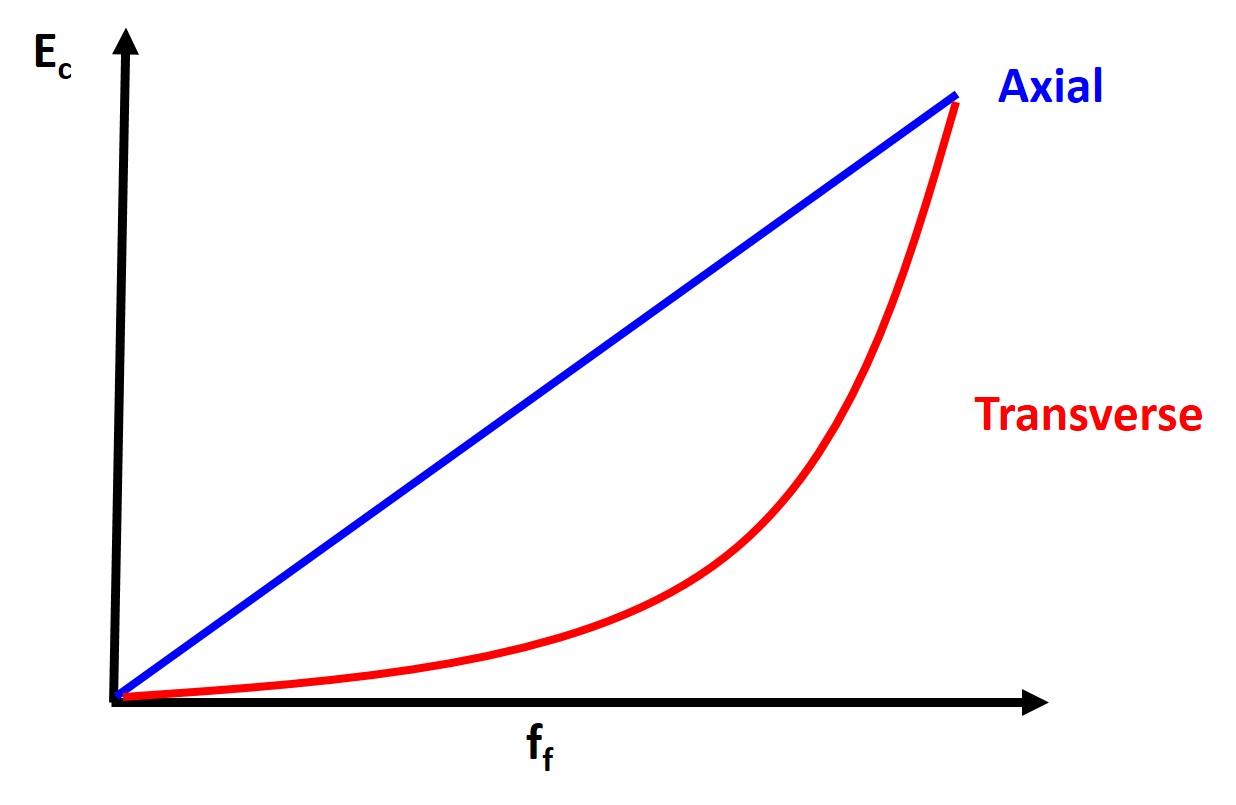
If we instead pull parallel to the fiber longitudinal or axial direction. Here the strain is the same but now the stresses will be different for the fibers and the matrix. So with those constraints we get

\begin{eqnarray}
\sigma_{c}=\sigma_{f}f_{f} + \sigma_{m}f_{m}\\
\epsilon_{c}=\epsilon_{m}=\epsilon_{f} \\
\sigma_{c} = E_{f}\epsilon f_{f} + E_{m}\epsilon f_{m}\\
E_{c} = E_{f}f_{f} + E_{m}f_{m}
\end{eqnarray}

We can see the difference in the Young’s modulus in both of these directions as function of volume fraction in the plot below

Composites are also useful tools to help blunt crack propagation.

6.4 Plastic Regime

Yielding Criterion:

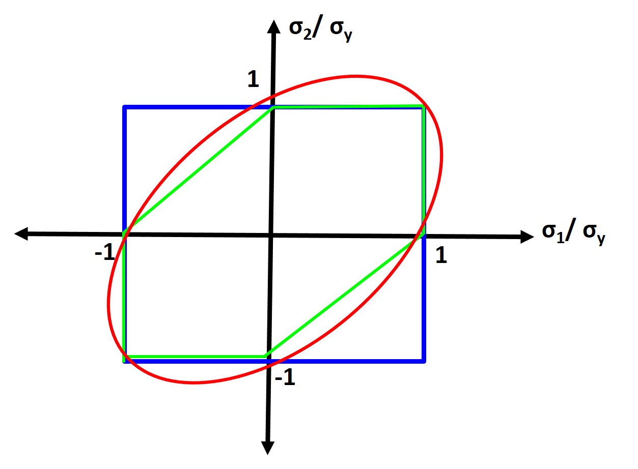
So far we have just been talking about stress and strain up to the yield point. However what happens beyond the elastic limit of materials? Well we have already discussed that the yield point denotes that the deformation is now permanent or plastic and we have initiated dislocation or defect motion. But as engineers perhaps the better or more useful question to ask is can we predict whether yielding will occur for materials that are not just simply loaded uniaxially. There are multiple yielding criterion that we will discuss, specifically: Rankine, Tresca, and von Mises Yield Criterion.

Rankine:

Rankine criterion also known as the maximum normal stress criterion states the a material will fail or yield when the maximal principal (normal) stress (σ₁) reaches the value where the material yields in uniaxial tension or compression so the material will yield when:

\begin{equation}
\sigma_{1}\geq\sigma_{y}
\end{equation}

Rankine doesn’t accurately describe material yielding, it is missing shear stress.

Tresca:

So let’s take a look at the Tresca criterion or the max shear stress criterion which states that the material yields when the \(\tau_{max}=\frac{\sigma_{1}-\sigma_{3}}{2}=\sigma_{y}\) reaches the value it does when material yields under uniaxial loading which is described below:

\begin{equation}
\sigma_{1}-\sigma_{3}\geq\sigma_{y}
\end{equation}

This is better, but in 1913 for WWI/WWII subs because they found that the Tresca criterion was a poor predictor for yielding.

Von Mises:

So we developed the Von Mises criterion is also called the maximum shear deformation energy (SDE) criterion and states the material will yield when the SDE reaches the yield stress value under uniaxial loading which is:

\begin{equation}
\sigma_{eff} = \sqrt{\frac{1}{2}[(\sigma_{11}-\sigma_{22})^2+(\sigma_{22}-\sigma_{33})^2+(\sigma_{33}-\sigma_{11})^2+6(\sigma^{2}_{23}+\sigma^{2}_{31}+\sigma^{2}_{12})]}\geq\sigma_{y}
\end{equation}

or in terms of the principal stresses:

\begin{equation}
\sigma_{eff} = \sqrt{\frac{1}{2}[(\sigma_{1}-\sigma_{2})^2+(\sigma_{2}-\sigma_{3})^2+(\sigma_{3}-\sigma_{1})^2]}\geq\sigma_{y}
\end{equation}

You can see by drawing the yield loci of these different criterion that Rankine is the most conservative yield criterion.

6.5 Yielding Mechanisms:

In a perfect copper crystal I can prove that the yield stress should be approximately 20GPa however the actual yield stress of copper is approximately 40MPa. What can explain the 3 order of magnitude difference? A nice approximation is that the theoretical yield stress is typically \(\frac{G}{30}\) and the theoretical fracture strength is \(\frac{E}{10}\).

Well remembering back to structure real materials have defects that allow atomic motion and in particular dislocation motion and slip a shear stress much lower than the theoretical prediction! We have talked quite a bit about the structure of dislocations but as of yet not too much about the motion of dislocations. What direction of motion will contribute most to yielding and dislocation motion?

The direction that require the least amount of energy to move! And remembering back to structure this corresponds to the shortest distance in your cell, i.e. the close paced planes and directions[9]. So for FCC the primary slip systems are the < 110 > directions and the 111 planes. For BCC it is the < 111 > directions and the 110 planes even though these aren’t close packed[9]. Remember as well that dislocations are also characterized by dislocation density which is again

\begin{equation}
\rho = \frac{N}{A}
\end{equation}

where N is the number of dislocations in a given area A. A material that is highly cold worked with a high dislocation density would be \(10^{14}\) dislocations per \(m^{2}\). A highly annealed material would exhibit a dislocation density closer to \(10^{7}\) dislocations per \(m^{2}\). You can also get a quick estimate of the distance between dislocations by the following relationship

\begin{equation}
\rho = \frac{1}{l^2}
\end{equation}

where l is the distance between dislocations!

6.6 Strengthening Mechanisms:

Now we have talked quite a bit about material constants and how they are often not really a constant. They vary depending on the material processing history! Perhaps no other material constant varies more depending on the processing history than yield stress. But as material scientists this gives us a fantastic knob to tune our materials for different applications. And the basic relationship to remember is that the yield stress increases when it becomes harder for dislocations to move or propagate. So when there are obstacles to dislocation motion the yield stress increases and we can do this via 4 primary mechanisms:

1. Work Hardening (more dislocations)
2. Solute Strengthening (more solute atoms)
3. Grain Size Strengthening (decrease grain size)
4. Precipitate/Particle Strengthening (add precipitates or particles)

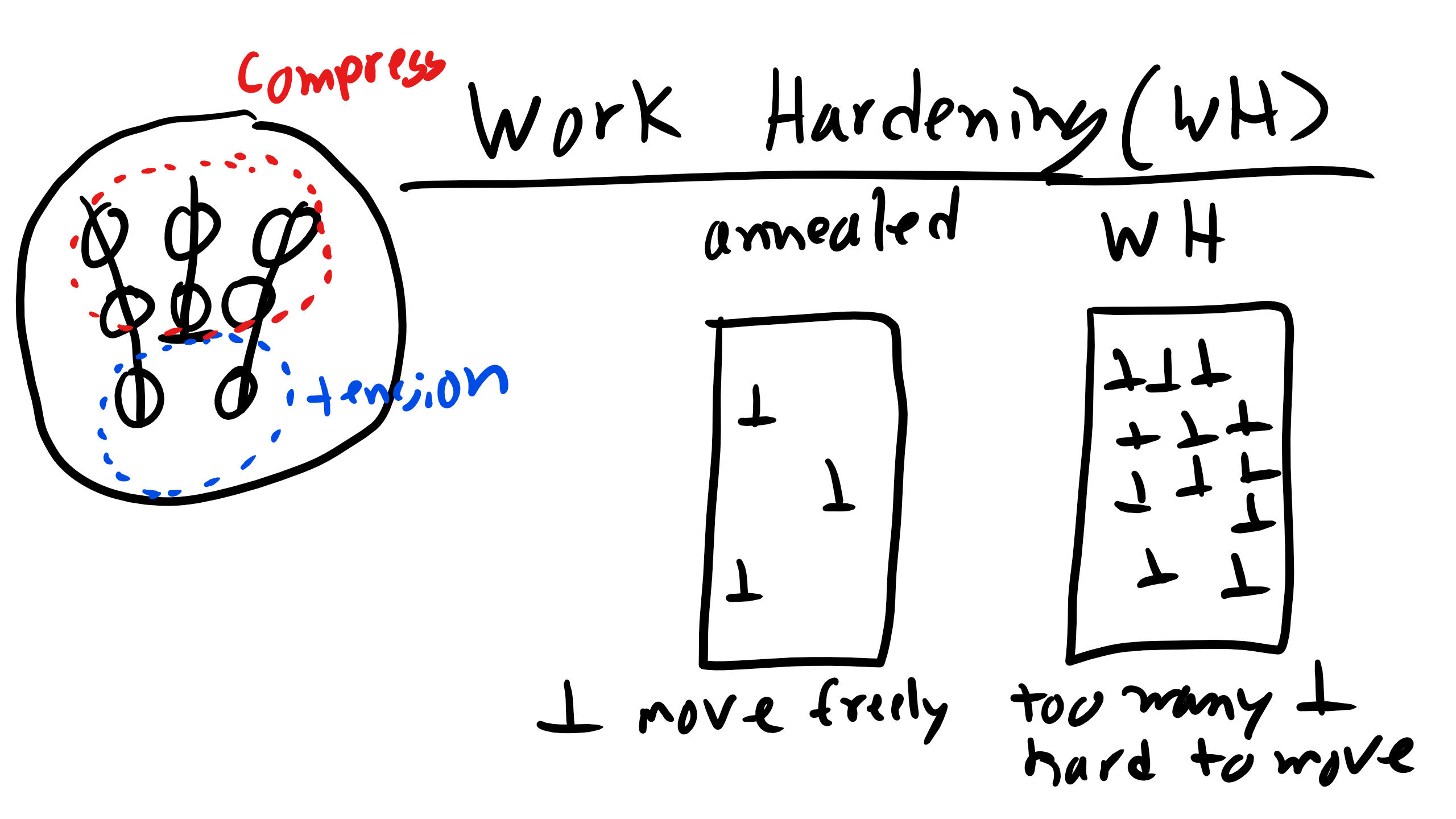
6.7 Work Hardening: Increase ρ via Plastic Deformation

\begin{equation}
\Delta \sigma_{y} = \alpha Gb\sqrt{\rho}
\end{equation}

where G is the shear modulus, b is Burgers vector, and α is the materials constant (close to 1). During the work hardening process you plastically deform the material and initiate or create dislocations in the material. This is often done in rolling sheet metal via cold-rolling. You create more dislocations which serve as obstacles for dislocation motion which then increases the yield strength as seen below

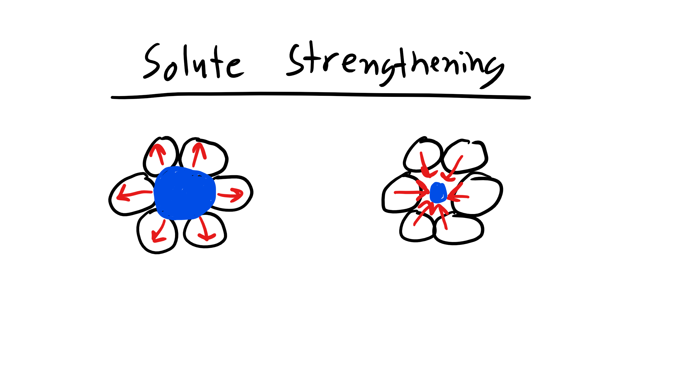
6.8 Solute Strengthening

\begin{equation}
\Delta \sigma_{y} = Gb\sqrt{c_{sol}}\epsilon^{\frac{3}{2}}_{sol}
\end{equation}

where \(c_{sol}\) is the concentration of the solute and \(\epsilon_{sol}\) is the lattice strain due to any size mismatch. We talked about this phenomenon a bit during structure. When you replace the a solvent atom with a larger solute atom you create a region with a localizes stress field that will interact with dislocation and again impede dislocation motion, causing yield stress to increase.

6.9 Grain Size Strengthening

\begin{equation}
\Delta \sigma_{y} = \frac{\kappa}{d_{g}}
\end{equation}

where \(\kappa\) is a materials constant and \(\d_g\) is the diameter of the grain. As you decrease the grain size there is less area for dislocation pile-up which is one method of reducing stress in your material. Smaller grain sizes can only accommodate so many dislocations before the dislocations can no longer pile up and they must be removed from the grain. It should be noted here the the yield stress does not blow up to infinity as the grain size shrinks to zero. Instead at about less than 10nm we see the yield stress begins to fall once again because now the grain is so small that only a single dislocation can fit inside a grain so you do not get enough dislocation pile-up.

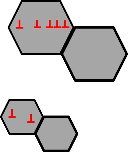
6.10 Precipitate/Particle Strengthening

In this case the obstacle to dislocation motion is not a point defect, a dislocation, or a grain boundary, but instead we have a new phase with a defined particle radius, spacing, and mechanical/structural properties. So when the dislocation encounters a defect the dislocation can do one of two things: 1.) Cut the precipitate/particle or 2.) Bow around the precipitates/particle. To cut through the particles we find the increase in yield stress to be:

\begin{equation}
\Delta \sigma_{y} = \frac{\gamma_{p-m} \pi r_{p}}{b l} = \kappa^{3} \sqrt{r_{p} f_{p}}
\end{equation}

where \(\gamma_{p-m} \) is the additional surface energy added when the particle is cut and thus is the surface energy of the particle/precipitate matrix, \(r_p\) is the radius of the particle, b is the burgers vector, l is the average particle spacing, \(\kappa\) is a materials constant, and \(f_p\) is the concentration or volume fraction of the particles.

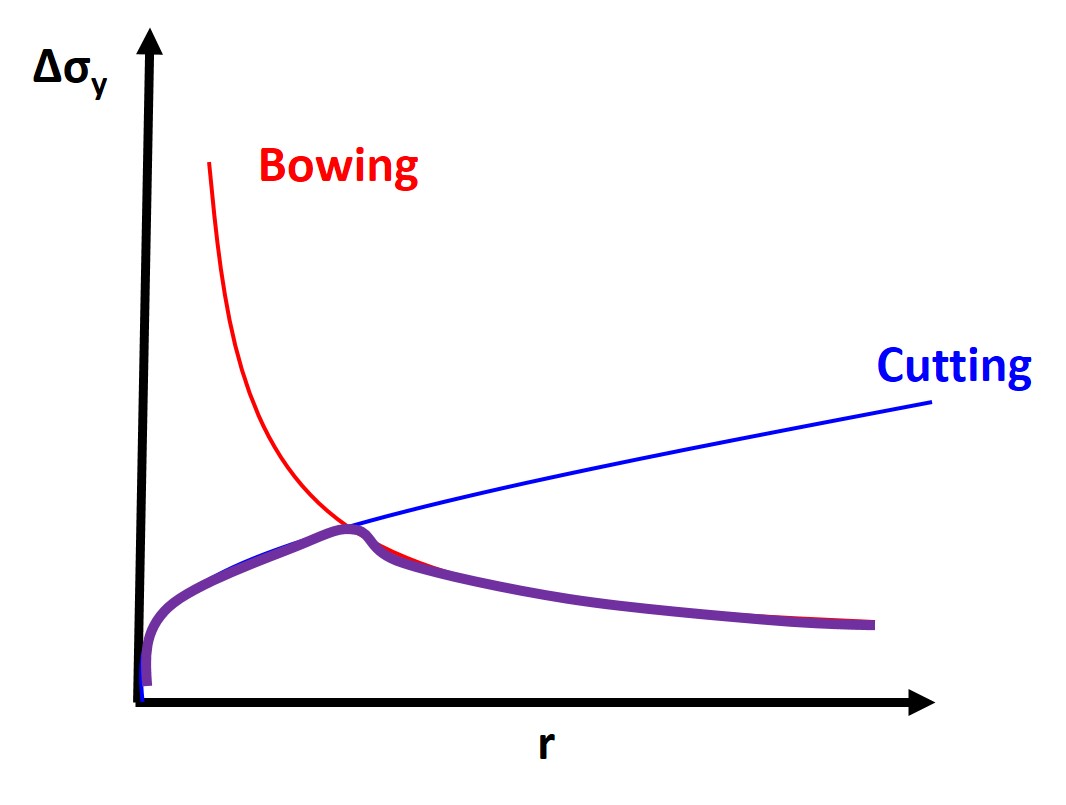
To bow around the precipitates/particle the increase in yield stress is

\begin{equation}
\Delta \sigma_{y} = \frac{Gb}{l-2r_{p}}
\end{equation}

where G is the shear modulus, b is the burgers vector, l is the average distance between particles and \(r_p\)is the radius of the particle. You can see energetically that at very small particle diameters it is more energetically favorable to cut the particles because the energy penalty of creating an increased surface is less for smaller particles. As the particles become larger bowing is more energetically favorable, for the same volume fraction of particles. As the volume fraction of particles or precipitates increases the critical radius for cutting vs. bowing decreases as you are now cutting even more particles which creates more surface area and an even larger energy penalty.

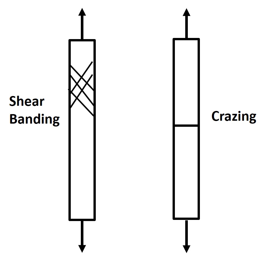
6.11 Polymer Yielding: Shear Banding and Crazing

Shear Banding:

Are zones of material alignment that are 1000s of nm wide and nucleate at stresses that are approximately 1000s of nms wide and continue to grow as stress exceeds. Shear band deformation is highly nonuniform. They are also not regions of high defect density but instead they are regions of chain alignment. Shear banding nucleation is also highly temperature dependent. Typically for uniaxial tension shear bands will form at 45^o relative to the applied stress(at locations of maximum shear stress).

Here is a good opportunity to talk about some asymmetry in yield criterion. Typically we find that the yield stress for uniaxial compression is larger than the yield stress for uniaxial tension. In polymers this is particularly true as tensile stress will tend to open up more free volume which makes it easier for chains to align.

Craze formation:

Also regions of highly localized deformation and they are distinct from a crack. Fibrils will span the craze. Crazes will form perpendicular to the loading axis with fibrils aligned with the loading axis. Crazing will not occur under compressive stress[9]. You can modify the von Mises criterion when considering shear banding and Tresca when considering crazing.

6.12 Time-Temperature Dependent Plasticity:

We have previously discussed creep in relation to polymer LVE. Creep is time or temperature dependent plastic deformation in crystalline materials. Creep is particularly insidious because like fatigue the stress where creep or fatigue ensues is much much less than the reported or measured yield stress of a material. This is because there are new plastic deformation mechanisms accessed at high T, high stress, and long times.

There are three typical creep regimes:

• Primary or Transient Creep

• Secondary or Steady State Creep

• Tertiary or Runaway Creep

Again as materials scientists we want to focus on predicting the creep strain rate, \(\dot{\epsilon_{c}}\)

\begin{equation}
\dot{\epsilon_{c}} = K_{c} \sigma^{x} d^{y}_{g} D_{c} = K_{c} \sigma^{x} d^{y}_{g} D_{o} \exp\bigg(\frac{-Q_{c}}{kT}\bigg)
\end{equation}

where \(K_c\) is an empirical material specific creep constant, \(\sigma\) is the applied stress, \(d_g\) is the grain diameter, and \(Q_c\) is the activation energy for that creep mechanism. Now those diffusion mechanisms are diffusion of vacancies through the lattice or bulk diffusivity, diffusion of vacancies along grain boundaries, and diffusion of vacancies to dislocations.

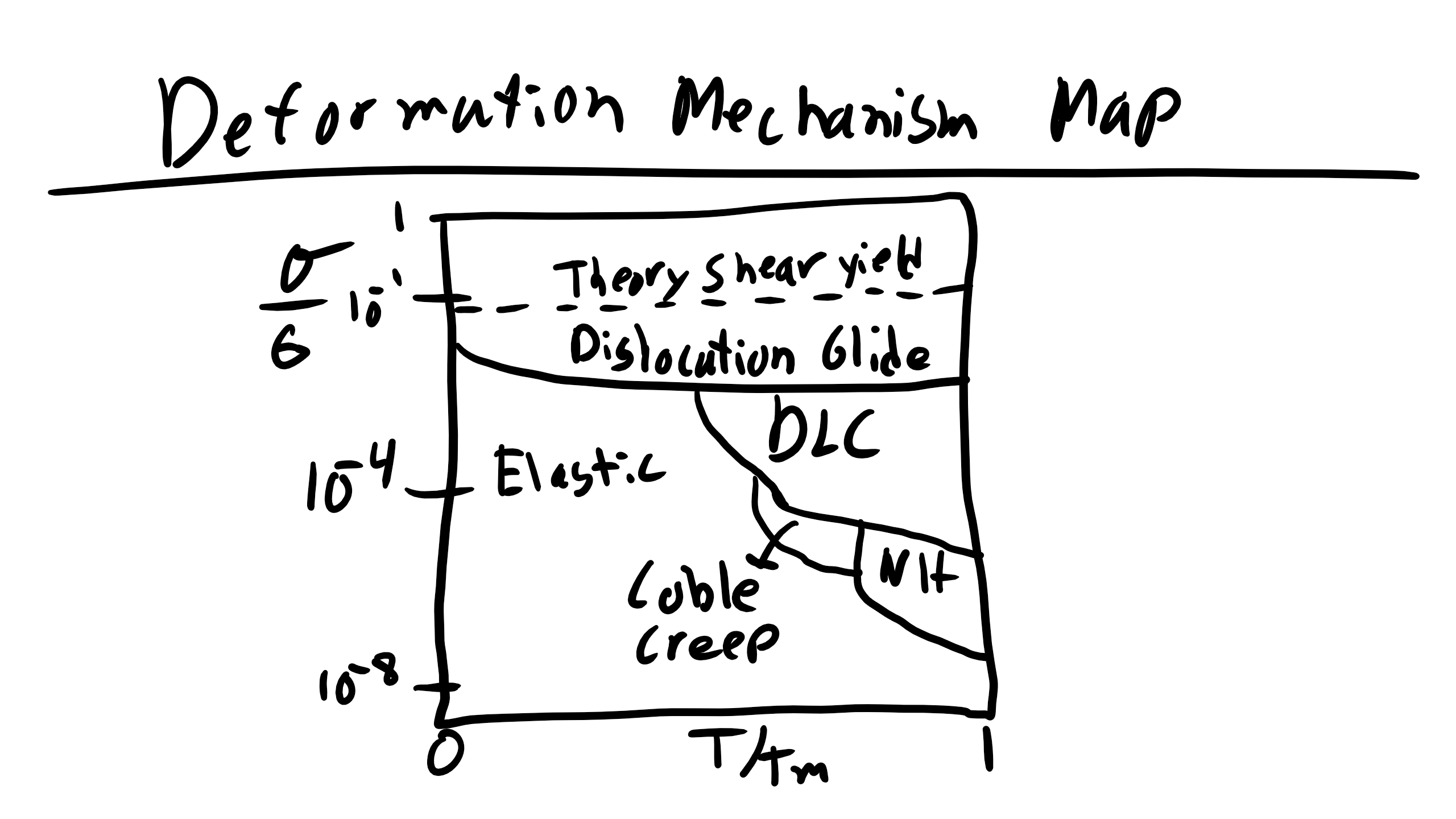
6.12.1 Lattice/Volume/Bulk Diffusion: Nabarro-Herring Creep

We have our equation for Nabarro-Herring Creep below:

\begin{equation}
\dot{\epsilon_{NH}} = \frac{K_{NH}\sigma D_{o} \exp\bigg(\frac{-Q_{L}}{kT}\bigg)}{d^{2}_{g}}
\end{equation}

the key things to see in this equation is the activation energy for lattice diffusion and the scaling behavior with the grain size.

6.12.2 Grain Boundary Diffusion: Coble Creep

Here the number of diffusive pathways increases as the grain size decreases and remember that the activation energy for grain boundary diffusion is lower than for bulk.

\begin{equation}
\dot{\epsilon_{CC}} = \frac{K_{CC}\sigma D_{o} \exp\bigg(\frac{-Q_{GB}}{kT}\bigg)}{d^{3}_{g}}
\end{equation}

6.12.3 Dislocation Creep or Power Law Creep

Here the net motion of dislocation cores moves in direction of applied stress, i.e. macroscopic creep. The dependence on applied stress is critical as you can see the scaling behavior in the equation below. Additionally dislocation climb is the rate-limiting process.

\begin{equation}
\dot{\epsilon_{DLC}} = K_{NH}\sigma^{4-6} D_{o} \exp\bigg(\frac{-Q_{L}}{kT}\bigg)
\end{equation}

We can now take a look at some key aspects of creep and in particular the scaling behavior of creep. We can see that DLC will dominate at high temperatures and high stress and Coble creep will dominate at lower temperatures compared to NH.

6.13 Fracture Regime

Finally Fracture!!

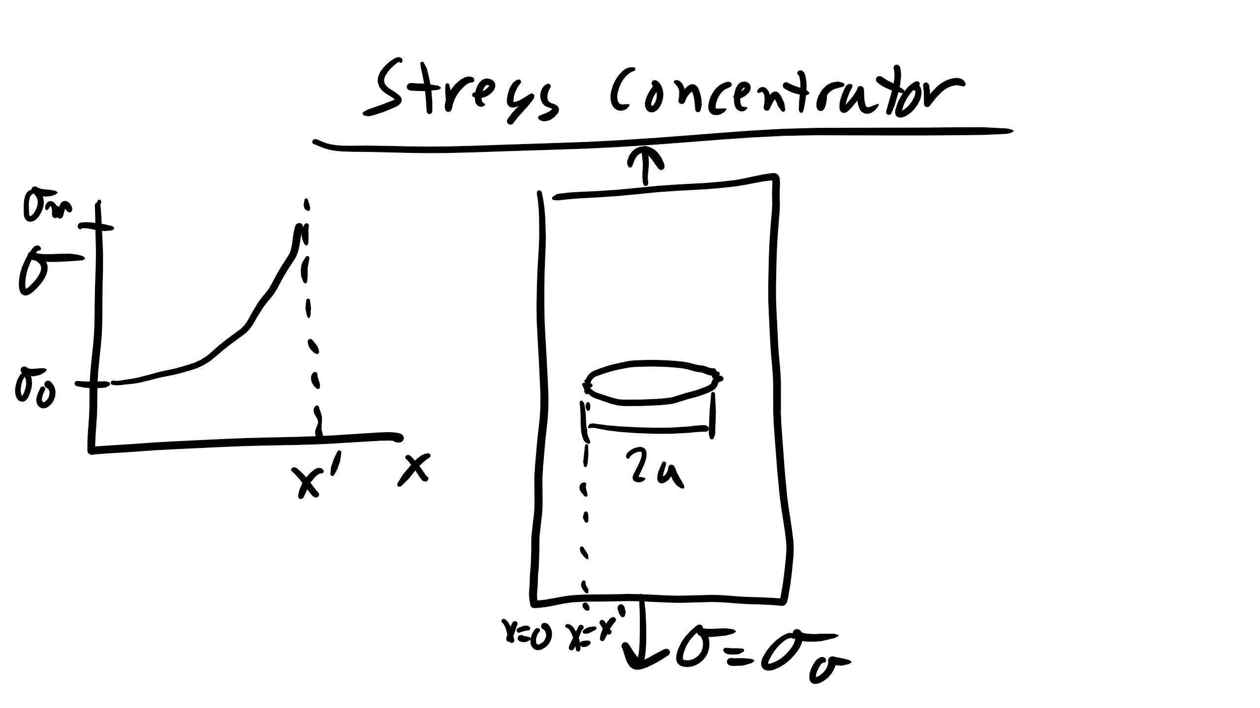
Fracture is the last resort for material deformation mechanisms when all other elastic/plastic mechanisms are exhausted. Energy is dissipated by bond breaking. In uniaxial loading, the stress required to break the material in two pieces, at the stress fracture. Again as in the case of yielding the theoretical stress required to fracture materials (Steel 4340 65GPa, Al 20GPA, Si 7GPA) is order of magnitudes lower than the actual stress required to fracture materials (Steel 4340-3GPa, Al .7GPA, Si .3GPA). This is because real materials typically contains cracks (inside, at surface, or at interfaces) and these micro-cracks act as stress concentrators. And for an elliptical hole we can define the stress as a function of the distance from the stress concentrator

\begin{equation}
\sigma = \sigma_{o}\bigg(1+2\sqrt{\frac{a}{R}}\bigg)
\end{equation}

and R at the tip of the crack is \(\frac{b^2}{a}\). Brittle fracture occurs when the stress concentrates at a pre-existing crack tip is so high that the material will break catastrophically.

Griffith’s Theory of Brittle Fracture:

We can develop an equation for brittle fracture from Griffith by considering the surface area created as the crack grows and relieving stored elastic energy.

Creating Surface Area as Crack Grows

To create the surface area of the crack as it grows we will have a change in the internal energy of the system

\begin{equation}
\Delta U_{surf} = 4at\gamma
\end{equation}

Relieving Stored Elastic Energy

A similar change in internal energy will occur for the the relieved stored elastic energy

\begin{equation}
\Delta U_{el} = -\frac{\pi a^{2} t \sigma^{2}}{2E}
\end{equation}

The crack will reach critical length when we minimize the total energy

\begin{equation}
\Delta U_{tot} = \Delta U_{surf} + \Delta U_{el} = 0
\end{equation}

Giving us the critical crack length

\begin{equation}
\sigma_{f} = \sqrt{\frac{2 \gamma E}{\pi a_{crit}}}
\end{equation}

6.13.1 Orowan Theory of Ductile Fracture:

There are a number of materials, metals and polymers, which won’t fracture in a completely brittle manner but instead from a small plastic zone prior to each crack elongation. For these materials Orowan has a theory for ductile fracture which is:

\begin{equation}
\sigma_{f} = \sqrt{\frac{E G_{c}}{\pi a}}
\end{equation}

where \(G_c\) the strain energy release rate.

6.13.2 Fracture Toughness:

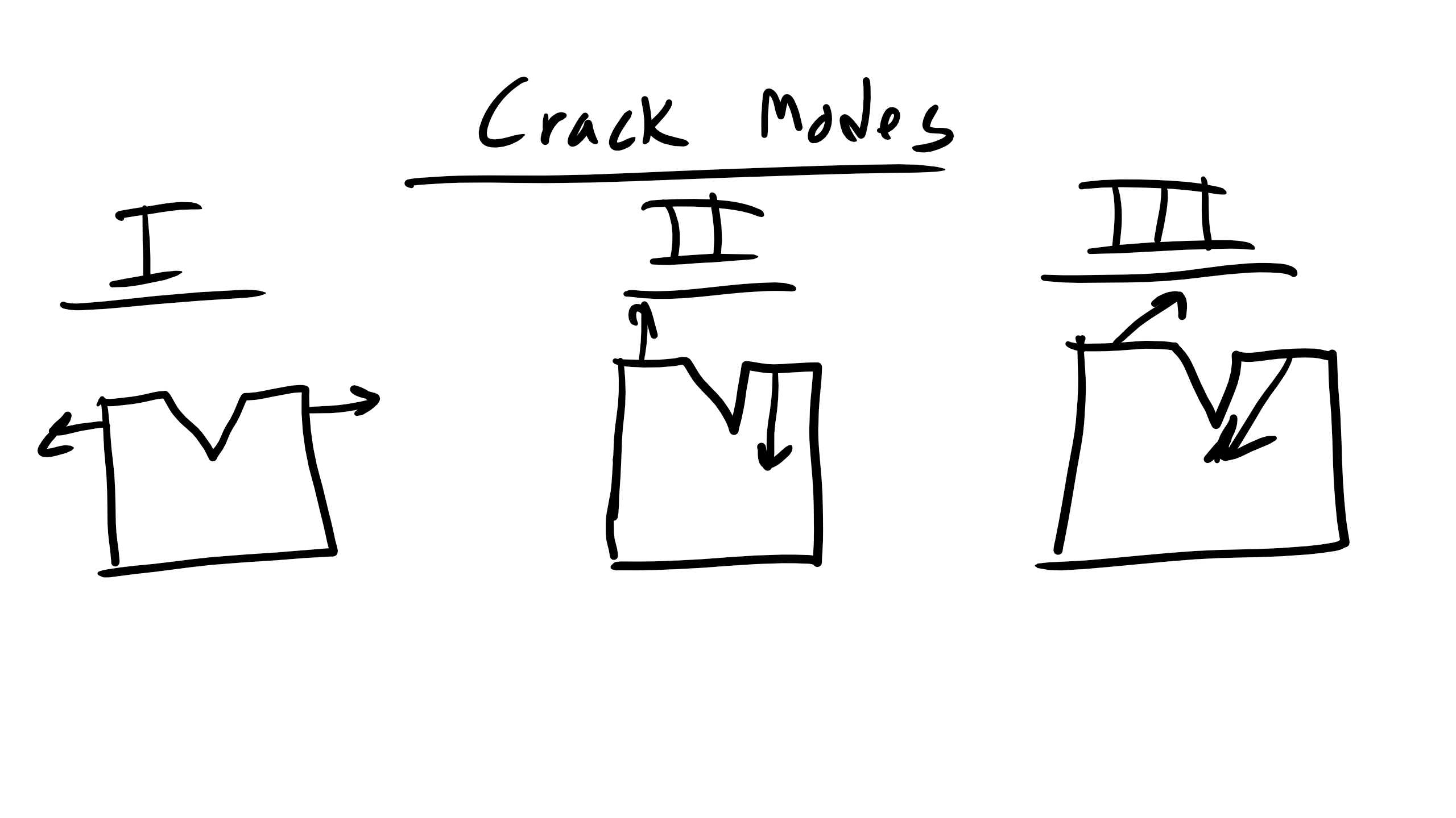
The final theory for fracture toughness considers when a material breaks when the stress intensity factor reaches a critical factor. The critical stress intensity factor depends on the mode of fracture: I, II, and III.

\begin{equation}
K_{c} = f \sigma \sqrt{\pi a}
\end{equation}

where f is a geometric constant factor and \(K_c\) is the fracture toughness and \(K_{I,II,III}\) is the critical stress intensity factor under Mode I, II, or II loading.

When one looks at the impact energy or fracture toughness as a function of temperature for brittle materials (like BCC which doesn’t have close packed slip planes) you will see a ductile to brittle fracture transition where the fracture toughness decreases dramatically as temperature decreases. For ductile materials like FCC which has a number of slip planes you will not see this sharp transition.

6.14 Fatigue

Fatigue (cyclic) loading occurs at applied stresses that are much much less than the stress at fracture but again like creep can lead to catastrophic failure at these low applied stresses.

Fatigue failure: fracture due to crack growth every cycle of loading or the crack growth increment per loading cycle which is defined below

\begin{equation}
\frac{da}{dn}
\end{equation}

where a is the crack length and n is the number of loading cycles.

We will deal with Static Fatigue and Cyclic or Classical Fatigue. Static fatigue occurs when a material is placed under a static or constant load and the crack faces of a material interacts with the environment, the crack tip becomes embrittled due to interaction with environment (stress corrosion cracking), the crack tip sharpens, the crack propagates, and the process repeats.

The more common fatigue scenario is cyclic or classical fatigue where a material is under a cyclic load/stress. We need to define the cyclic applied stress specifically the frequency of the applied load, f, which is where \(\tau\) is the period of the applied stress. We also want to quantify the stress ratio, R

\begin{equation}
R = \frac{\sigma_{min}}{\sigma_{max}}
\end{equation}

As materials scientists we want to avoid catastrophic failure and for fatigue that involves trying to estimate the number of cycles to failure, \(N_f\), which is the number of cycles to grow a crack from initial length, \(a_o\), to the critical or catastrophic crack length, \(a_c\).

There three distinct regimes of fatigue crack growth: I) The Slow-Growth Rate or NearThreshold Regime, II) Mid-Growth Rate or the Paris Regime, and III) High-Growth

Rate Regime

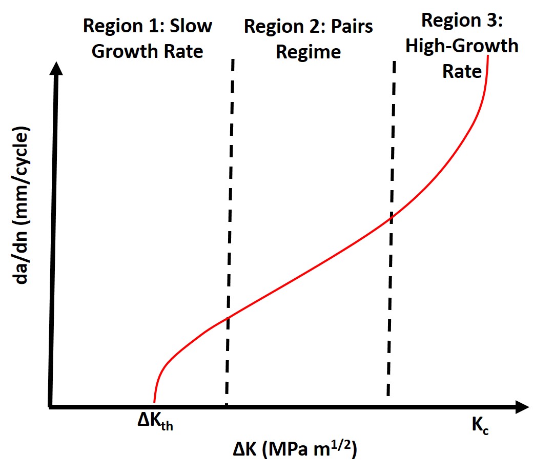
I) Slow-Growth Rate or Near-Threshold Regime

In the slow-growth rate regime the crack won’t grow initially until the threshold stress intensity factor, \(\Delta K\), is reached where

\begin{equation}
\Delta K = f \Delta \sigma \sqrt{\pi a}
\end{equation}

Typically we say that when the rate of crack growth is \(10^{-8}\) mm/cycle or less the crack is dormant or growing a a near undetectable rate. Once the threshold stress intensity factor is reached the crack growth rate will increase but still the growth rate is extremely slow, still below one lattice spacing per cycle until we reach the Mid-Growth Rate or the Pairs Regime.

II) Mid-Growth Rate or Paris Regime

In the Mid-Growth Rate or Paris Regime we actually have an equation or law to describe fatigue crack growth, aptly named the Paris Law:

\begin{equation}
\frac{da}{dN} = C\Delta K^{m}
\end{equation}

where C and are empirical constants which depend on the material, the applied stress, frequency, and R. We can use Paris law to predict the number of cycles to failure, \(N_f\)
\begin{equation}
\int^{N_{F}}_{0}dN = \int^{a_{c}}_{a_{o}} \frac{da}{C(f \Delta \sigma \sqrt{\pi a})^m}
\end{equation}

which leads to

\begin{equation}
N_{f} = \frac{1}{C(f \Delta \sigma \sqrt{\pi})^m} \bigg[\frac{a^{1-\frac{m}{2}}_{c} - a^{1-\frac{m}{2}}_{o}}{1- \frac{m}{2}}\bigg]
\end{equation}

where \(a_o\) is the initial crack length and remember that \(a_c\)

\begin{equation}
a_{c} = \frac{1}{\pi} \bigg(\frac{K_{IC}}{\sigma_{max}}\bigg)^2
\end{equation}

Fatigue cracks are marked via striations on the fracture surface.

III) High-Growth Rate Regime

The last stage is the high-growth rate regime is characterized by an orders of magnitude increase in the crack growth rate and additional cleavage in the material or microvoid coalescence. This is the end region where catastrophic crack failure will occur throughout the material. We need to take the material out of service before we reach this regime.

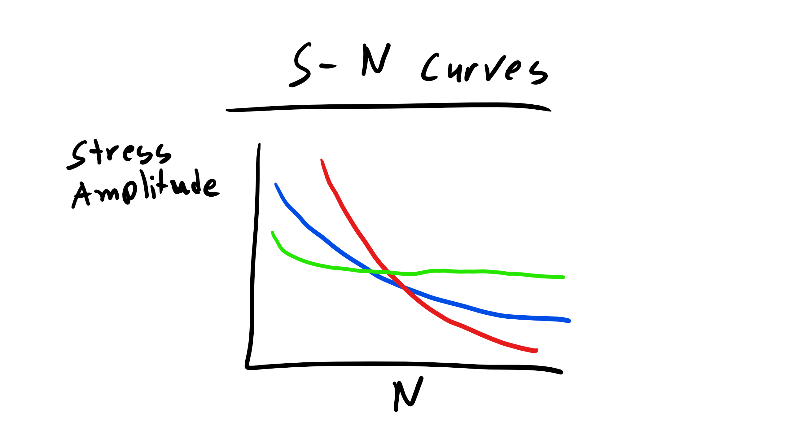
One way that we can try to predict the lifetime of materials is by looking at empirically determined S-N curves. S is the stress amplitude so the difference between the maximum and minimum applied stress. N is again the number of cycles. We can look at the curve and determine when the material will fail.