
Chapter 5: Mechanical Behavior of Materials Part I
- Page ID
- 97983

\( \newcommand{\vecs}[1]{\overset { \scriptstyle \rightharpoonup} {\mathbf{#1}} } \)
\( \newcommand{\vecd}[1]{\overset{-\!-\!\rightharpoonup}{\vphantom{a}\smash {#1}}} \)
\( \newcommand{\dsum}{\displaystyle\sum\limits} \)
\( \newcommand{\dint}{\displaystyle\int\limits} \)
\( \newcommand{\dlim}{\displaystyle\lim\limits} \)
\( \newcommand{\id}{\mathrm{id}}\) \( \newcommand{\Span}{\mathrm{span}}\)
( \newcommand{\kernel}{\mathrm{null}\,}\) \( \newcommand{\range}{\mathrm{range}\,}\)
\( \newcommand{\RealPart}{\mathrm{Re}}\) \( \newcommand{\ImaginaryPart}{\mathrm{Im}}\)
\( \newcommand{\Argument}{\mathrm{Arg}}\) \( \newcommand{\norm}[1]{\| #1 \|}\)
\( \newcommand{\inner}[2]{\langle #1, #2 \rangle}\)
\( \newcommand{\Span}{\mathrm{span}}\)
\( \newcommand{\id}{\mathrm{id}}\)
\( \newcommand{\Span}{\mathrm{span}}\)
\( \newcommand{\kernel}{\mathrm{null}\,}\)
\( \newcommand{\range}{\mathrm{range}\,}\)
\( \newcommand{\RealPart}{\mathrm{Re}}\)
\( \newcommand{\ImaginaryPart}{\mathrm{Im}}\)
\( \newcommand{\Argument}{\mathrm{Arg}}\)
\( \newcommand{\norm}[1]{\| #1 \|}\)
\( \newcommand{\inner}[2]{\langle #1, #2 \rangle}\)
\( \newcommand{\Span}{\mathrm{span}}\) \( \newcommand{\AA}{\unicode[.8,0]{x212B}}\)
\( \newcommand{\vectorA}[1]{\vec{#1}} % arrow\)
\( \newcommand{\vectorAt}[1]{\vec{\text{#1}}} % arrow\)
\( \newcommand{\vectorB}[1]{\overset { \scriptstyle \rightharpoonup} {\mathbf{#1}} } \)
\( \newcommand{\vectorC}[1]{\textbf{#1}} \)
\( \newcommand{\vectorD}[1]{\overrightarrow{#1}} \)
\( \newcommand{\vectorDt}[1]{\overrightarrow{\text{#1}}} \)
\( \newcommand{\vectE}[1]{\overset{-\!-\!\rightharpoonup}{\vphantom{a}\smash{\mathbf {#1}}}} \)
\( \newcommand{\vecs}[1]{\overset { \scriptstyle \rightharpoonup} {\mathbf{#1}} } \)
\(\newcommand{\longvect}{\overrightarrow}\)
\( \newcommand{\vecd}[1]{\overset{-\!-\!\rightharpoonup}{\vphantom{a}\smash {#1}}} \)
\(\newcommand{\avec}{\mathbf a}\) \(\newcommand{\bvec}{\mathbf b}\) \(\newcommand{\cvec}{\mathbf c}\) \(\newcommand{\dvec}{\mathbf d}\) \(\newcommand{\dtil}{\widetilde{\mathbf d}}\) \(\newcommand{\evec}{\mathbf e}\) \(\newcommand{\fvec}{\mathbf f}\) \(\newcommand{\nvec}{\mathbf n}\) \(\newcommand{\pvec}{\mathbf p}\) \(\newcommand{\qvec}{\mathbf q}\) \(\newcommand{\svec}{\mathbf s}\) \(\newcommand{\tvec}{\mathbf t}\) \(\newcommand{\uvec}{\mathbf u}\) \(\newcommand{\vvec}{\mathbf v}\) \(\newcommand{\wvec}{\mathbf w}\) \(\newcommand{\xvec}{\mathbf x}\) \(\newcommand{\yvec}{\mathbf y}\) \(\newcommand{\zvec}{\mathbf z}\) \(\newcommand{\rvec}{\mathbf r}\) \(\newcommand{\mvec}{\mathbf m}\) \(\newcommand{\zerovec}{\mathbf 0}\) \(\newcommand{\onevec}{\mathbf 1}\) \(\newcommand{\real}{\mathbb R}\) \(\newcommand{\twovec}[2]{\left[\begin{array}{r}#1 \\ #2 \end{array}\right]}\) \(\newcommand{\ctwovec}[2]{\left[\begin{array}{c}#1 \\ #2 \end{array}\right]}\) \(\newcommand{\threevec}[3]{\left[\begin{array}{r}#1 \\ #2 \\ #3 \end{array}\right]}\) \(\newcommand{\cthreevec}[3]{\left[\begin{array}{c}#1 \\ #2 \\ #3 \end{array}\right]}\) \(\newcommand{\fourvec}[4]{\left[\begin{array}{r}#1 \\ #2 \\ #3 \\ #4 \end{array}\right]}\) \(\newcommand{\cfourvec}[4]{\left[\begin{array}{c}#1 \\ #2 \\ #3 \\ #4 \end{array}\right]}\) \(\newcommand{\fivevec}[5]{\left[\begin{array}{r}#1 \\ #2 \\ #3 \\ #4 \\ #5 \\ \end{array}\right]}\) \(\newcommand{\cfivevec}[5]{\left[\begin{array}{c}#1 \\ #2 \\ #3 \\ #4 \\ #5 \\ \end{array}\right]}\) \(\newcommand{\mattwo}[4]{\left[\begin{array}{rr}#1 \amp #2 \\ #3 \amp #4 \\ \end{array}\right]}\) \(\newcommand{\laspan}[1]{\text{Span}\{#1\}}\) \(\newcommand{\bcal}{\cal B}\) \(\newcommand{\ccal}{\cal C}\) \(\newcommand{\scal}{\cal S}\) \(\newcommand{\wcal}{\cal W}\) \(\newcommand{\ecal}{\cal E}\) \(\newcommand{\coords}[2]{\left\{#1\right\}_{#2}}\) \(\newcommand{\gray}[1]{\color{gray}{#1}}\) \(\newcommand{\lgray}[1]{\color{lightgray}{#1}}\) \(\newcommand{\rank}{\operatorname{rank}}\) \(\newcommand{\row}{\text{Row}}\) \(\newcommand{\col}{\text{Col}}\) \(\renewcommand{\row}{\text{Row}}\) \(\newcommand{\nul}{\text{Nul}}\) \(\newcommand{\var}{\text{Var}}\) \(\newcommand{\corr}{\text{corr}}\) \(\newcommand{\len}[1]{\left|#1\right|}\) \(\newcommand{\bbar}{\overline{\bvec}}\) \(\newcommand{\bhat}{\widehat{\bvec}}\) \(\newcommand{\bperp}{\bvec^\perp}\) \(\newcommand{\xhat}{\widehat{\xvec}}\) \(\newcommand{\vhat}{\widehat{\vvec}}\) \(\newcommand{\uhat}{\widehat{\uvec}}\) \(\newcommand{\what}{\widehat{\wvec}}\) \(\newcommand{\Sighat}{\widehat{\Sigma}}\) \(\newcommand{\lt}{<}\) \(\newcommand{\gt}{>}\) \(\newcommand{\amp}{&}\) \(\definecolor{fillinmathshade}{gray}{0.9}\)5.1 Sign Conventions
Sign Conventions:
To begin let’s talk about units and sign conventions. We will define any forces, stresses, or strain in tension as positive and any forces, stresses, or strain under compression will be considered negative. Additionally we will consider moments that are counter clockwise as positive and clockwise as negative.
There are a series of recorded lecture videos to supplement this text which can be seen in the playlist here:
5.2 Stress-Strain Curve:
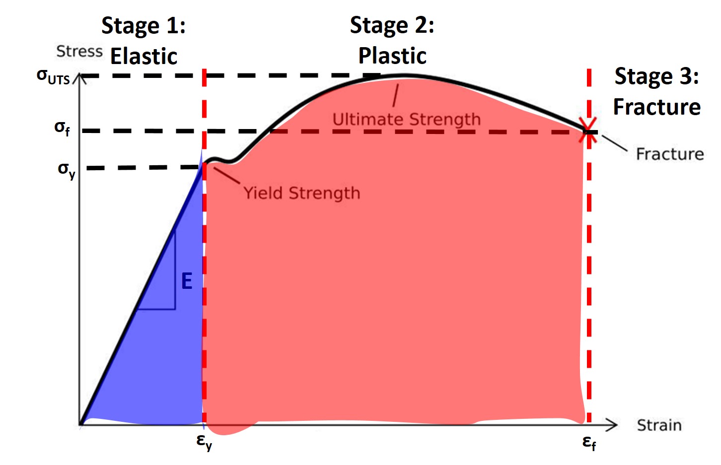
When a material is placed under a stress state we will typically plot a stress-strain curve and that curve typically will have 3 distinct regions: I) Elastic, II) Plastic, III) Fracture.
I) Elastic Regime:
In the elastic regime the stress strain response is linear and defined by the expression below which should be familiar (Hooke’s Law):
\begin{equation}
\sigma = E\epsilon
\end{equation}
where E, sometimes Y, is defined as the Young’s Modulus. It describes the stiffness of the material and is a material constant. Metals are typically in the 100s of GPa, ceramics are high 200’s and 300’s of GPa, polymers are closer to on the order of 1 GPa. In the elastic region the strain is completely reversible, i.e. there is no permanent or plastic deformation. You are just pulling on the bonds not breaking any bonds.
II) Plastic Regime:
Here you are plastically deforming the material and this is signified microstructurally by the breaking of bonds and the movement of dislocations[9]. Additionally with plastic dislocation the strain is not reversible, if you remove the force the strain remains. It is signified to begin on the stress strain curve by \(\sigma_y\) which is the yield stress and \(\epsilon_y\) the yield strain. The \(\sigma_{UTS}\) is the ultimate tensile strength and it denotes the onset of necking which is where the instantaneous area is now smaller than the original area.
III) Fracture:
As the name denotes this is where the material catastrophically fractures and is denoted by \(\sigma_f\) which is the fracture stress and the \(\epsilon_f\) the fracture strain.
At this point we need to stop and make a clear point about the language that we have to use when discussing the material properties of materials. Word choice is critical here because they mean very different things. When we talk about the stiffness of materials we are talking about the Young’s modulus of the material. The higher the Young’s modulus the stiffer the material. When we talk about strength we are talking about the yield strength, the ultimate tensile strength, or the fracture stress or strength. We we are talking about how ductile a material is we are talking about the strain at failure. We also often talk about material resilience and toughness as well.
We define elastic strain energy (ESE) which is defined as:
\begin{equation}
U_{ESE} = V \int^{\epsilon_{y}}_{0}\sigma_{11} d\epsilon_{11}
\end{equation}
where V is the volume which gives us units of energy. This is the blue shaded portion. Toughness is defined as
\begin{equation}
U_{T} = V \int^{\epsilon_{f}}_{0}\sigma_{11} d\epsilon_{11}
\end{equation}
If a material is not as stiff it is called compliant, if a material is not strong it is weak, and if a material is not tough it is termed brittle.
Let’s look at a couple of stress strain curves...
5.3 Elastic Regime:
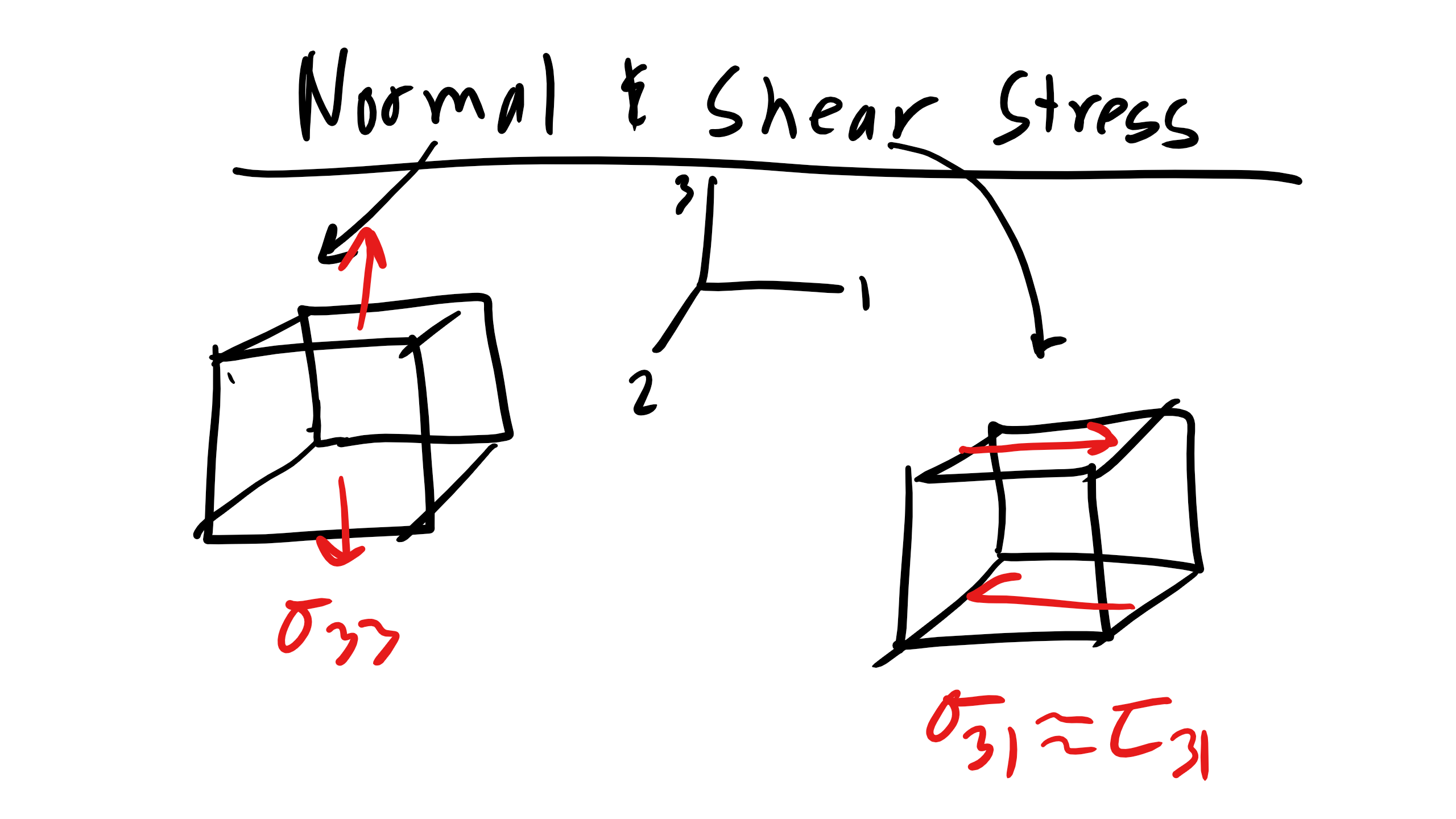
Stress, \(\sigma\), is a force normalized by the area over which it acts and the force is perpendicular to the area:
\begin{equation}
\sigma = \frac{F}{A} = \frac{N}{m^2} = Pa
\end{equation}
where F is force and A is the original area. This is the definition of the engineering stress the true stress would be normalized by the instantaneous area. In this class we will use the engineering stress primarily in this class. Shear stress, \(\tau\), is a force normalized by the area over which it acts and the force is parallel to the area.
The shear stress is similarly defined as:
\begin{equation}
\tau = \frac{F}{A}
\end{equation}
Now it should be noted here that stress is a second rank tensor, \(\sigma_{ij}\), and so is strain, \(\epsilon_{ij}\). For stress i denotes the normal to the plane, on which the force is acting and j is the direction of the force:
\begin{equation}
\sigma_{ij} = \frac{F_{j}}{A_{i}}
\end{equation}
So our full stress tensor or our most generic stress state would be:
\begin{equation}
\sigma =
\begin{bmatrix}
\sigma_{11} & \sigma_{12} & \sigma_{13} \\
\sigma_{21} & \sigma_{22} & \sigma_{23} \\
\sigma_{31} & \sigma_{32} & \sigma_{33} \\
\end{bmatrix}
\end{equation}
Now this looks like a complex matrix with 9 independent components however they are not completely independent. If we assume that our cube volume element (representative volume element (RVE) is in equilibrium (not rotating) then we have the condition that
\begin{eqnarray}
\sigma_{12} = \sigma_{21}\\
\sigma_{23} = \sigma_{32}\\
\sigma_{31} = \sigma_{13}
\end{eqnarray}
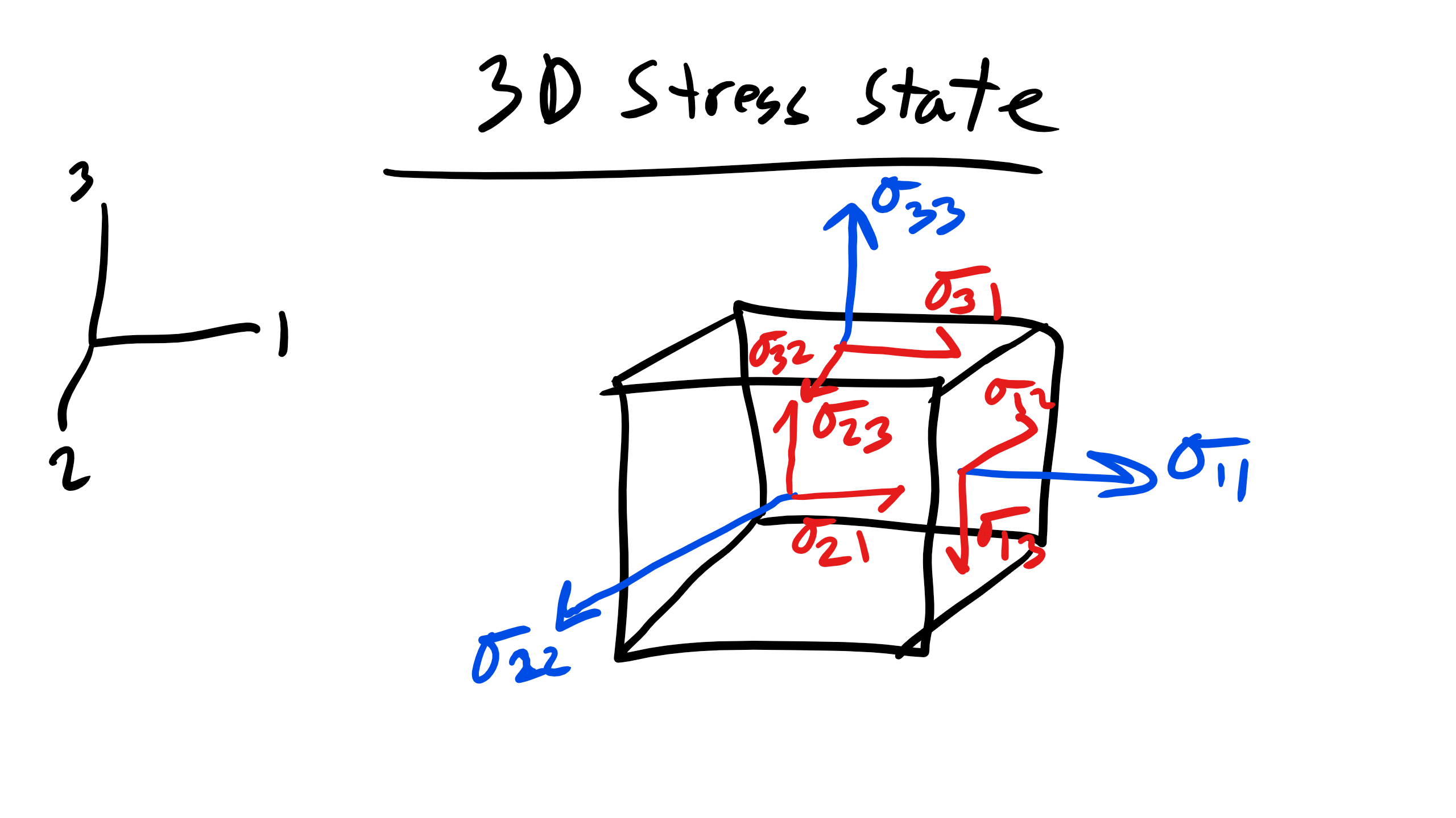
so our matrix reduces to 6 independent components for our RVE
\begin{equation}
\sigma =
\begin{bmatrix}
\sigma_{11} & \sigma_{12} & \sigma_{13} \\
\sigma_{12} & \sigma_{22} & \sigma_{23} \\
\sigma_{13} & \sigma_{23} & \sigma_{33} \\
\end{bmatrix}
\end{equation}
Additionally we will encounter several special stress states like Uniaxial stress which gives the following stress state
\begin{equation}
\sigma =
\begin{bmatrix}
\sigma_{11} & 0 & 0 \\
0 & 0 & 0 \\
0 & 0 & 0 \\
\end{bmatrix}
\end{equation}
and Biaxial stress which gives us
\begin{equation}
\sigma =
\begin{bmatrix}
\sigma_{11} & \sigma_{12} &0 \\
\sigma_{12} & \sigma_{22} & 0 \\
0 & 0 & 0 \\
\end{bmatrix}
\end{equation}
but more on those a bit later. Additionally we define the hydrostatic stress as
\begin{equation}
P = \frac{1}{3} (\sigma_{11} + \sigma_{22} + \sigma_{33})
\end{equation}
5.4 Strain:
All machines, structural members, and materials will deform to some extend when externally loaded by a force or stress. That deformation results in a displacement or strain, \(\epsilon\)
\begin{equation}
\epsilon = \frac{dL}{L}
\end{equation}
\begin{equation}
\epsilon_{t} = \int_{L_1}^{L_2} \frac{dL}{L} = ln \frac{L_{2}}{L_{1}}
\end{equation}
where \(L_1\) is the original length. This is the definition of true strain, \(\epsilon\), but typically we work with a simpler form called the engineering strain, \(\epsilon_e\)
\begin{equation}
\epsilon_{e} = \frac{L_{2}-L_{1}}{L_{1}} = \frac{\Delta L}{L_{1}}
\end{equation}
Typically engineers work with microstrain or parts per million. And the shear strain is:
\begin{equation}
\gamma = \frac{dx}{y = \tan \theta
\end{equation}
as seen in the figure below

Also for a material subjected to shear stresses we observe a proportional relationship between shear stress and strain in the elastic regime which is defined as:
\begin{equation}
\tau = G \gamma
\end{equation}
where G is the shear modulus.
Poisson’s Ratio:
Now what happens to the dimensions perpendicular to the direction of applied force when a the material is subjected to uniaxial tension? We know from experience that a body begin pulled in tension will contract laterally. This lateral strain is described by the Poisson’s Ratio:
\begin{equation}
\nu = -\frac{\epsilon_{L}}{\epsilon_{A}}
\end{equation}
where \(\epsilon_L\)is the lateral strain and \(\epsilon_A\) is the axial strain. Note the negative sign which signifies a decrease in length. The Poisson’s ratio is typically around 0.3 for metals, 0.5 for rubber, 0.4-0.5 for polymeric materials or biomaterials, and 0.2 for cork, cellular materials, or ceramics.
5.5 Biaxial and Complex Stress States:
What happens when we have a more complex stress state and we are interested in the stress state of a particular plane of orientation angle θ? Well we do this the same way we resolve force vectors onto a new axes of interest. Let’s look at a case of plane stress which is a case when all the stress is contained in one plane.
So far we have been dealing with simple uniaxial stress along the principal testing direction however often materials can also be subjected to shear stress or strain.
With this information let us move on to more complex stress states, specifically one that typically exists on a free, not constrained, surface of a stressed material.
Consider the element which is initially stressed in the 1 direction by applying \(\sigma_{11}\). There will be a resultant strain:
\begin{eqnarray}
\epsilon_{11} = \frac{\sigma_{11}}{E}\\
\epsilon_{22} = \frac{-\nu \sigma_{11}}{E}
\end{eqnarray}
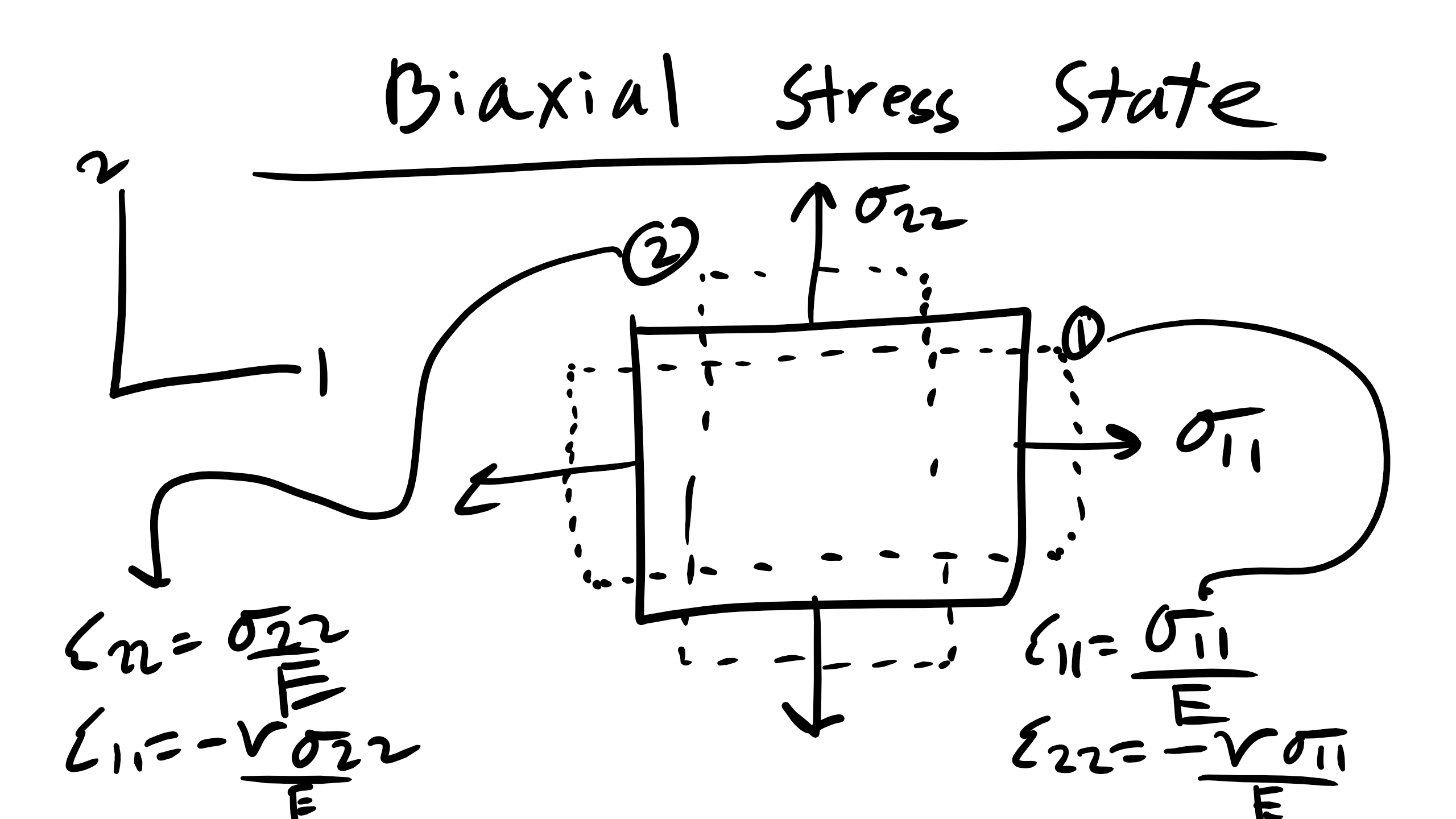
Figure \(\PageIndex{5}\): Biaxial Stress State
The element is then stressed in the 2 direction by applying \(\sigma_{22}\). The resultant strain will be:
\begin{eqnarray}
\epsilon_{22} = \frac{\sigma_{22}}{E}\\
\epsilon_{11} = \frac{-\nu \sigma_{22}}{E}
\end{eqnarray}
therefore the total strain in 1 and 2 directions will be:
\begin{eqnarray}
\epsilon_{11} = \frac{\sigma_{11} - \nu \sigma_{22}}{E}\\
\epsilon_{22} = \frac{\sigma_{22} - \nu \sigma_{11}}{E}
\end{eqnarray}
3D Stress State
\begin{eqnarray}
\epsilon_{11} = \frac{1}{E} [\sigma_{11} - \nu(\sigma_{22} + \sigma_{33})]\\
\epsilon_{22} = \frac{1}{E} [\sigma_{22} - \nu(\sigma_{33} + \sigma_{11})]\\
\epsilon_{33} = \frac{1}{E} [\sigma_{33} - \nu(\sigma_{11} + \sigma_{22})]
\end{eqnarray}
5.6 Thermal Expansion Coefficient
Let’s go back once again to our gold old friend the LJ potential when temperature increases we know that the thermal energy increases, causing the atoms to vibrate and oscillate around their equilibrium distance ro. Now if the potential was symmetric or harmonic (like at the minimum of a quadratic function) then the atoms would equally be distributed at distances less than or greater than the the equilibrium distance. However, as you can see the LJ and most atomic potentials are asymmetric or anharmonic and thus when the atoms fluctuate they will tend to occupy positions with the lowest energy and one can see that as temperature increase and as the molecules deviate further and further from their equilibrium position they will tend to adopt positions with lower energies. Thus, as you can see on average the molecules will tend to expand because the larger interatomic distances have lower energies and thus the materials will tend to expand.

So to put it simply at \(T = 0K\)the atoms will be at their equilibrium distance \(r_o\) and then as temperature increase the atoms will essentially move up the anharmonic potential to lower their energy. The equilibrium distance thus shifts to the right depending on the thermal expansion coefficient \(\alpha\) and thus we can write this thermally induced strain as
\begin{equation}
\epsilon_{T} = \alpha \Delta T
\end{equation}
Now for linear elastic isotropic materials the material will expand uniformly in all directions and there will be no shear strain from thermal expansion. Some typical thermal expansion coefficients for some materials can be seen below, all \(\times 10^{-6} K^{-1}\)
• Polymers 50-500
• Metals 5-50
• Ceramics 1-10
• Glasses 1-2
Taking into account thermal strain is incredibly important in and in many materials processes when you heat a material that is a composite and cool it can induce residual stresses due to the incompatible thermal strains.
It should be noted that thermal strain will only occur along normal directions and you must add it on to the expression for strain if there is a change in temperature during your operation.
5.7 General Linear Elastic Isotropic Cubic Material Stress and Strain Expression
To write the most general expression of stress and strain for linear elastic isotropic cubic materials and thermal expansion
\begin{equation}
\epsilon_{ij} = \frac{1}{E} \bigg [ (1+\nu)\sigma_{ij} - \nu \sigma_{kk} \delta_{ij} \bigg]+\alpha \Delta T \delta_{ij}
\end{equation}
where \(\delta_{ij}\) is the Kronecker Delta which will be 1 when \(i=j\) and 0 when \(i \neq j\)
5.7.1 Ex. Jewelry Maker: Strain Without Stress?
A jewelry maker creates a die to form a new cufflink made of steel. We need to know how much stress to apply to the metal slab to reduce the thickness to 3mm. The die is a simple channel that does not constrain the metal in the x-direction and the channel is well lubricated so that all frictional forces and stresses along the channel walls can be ignored.
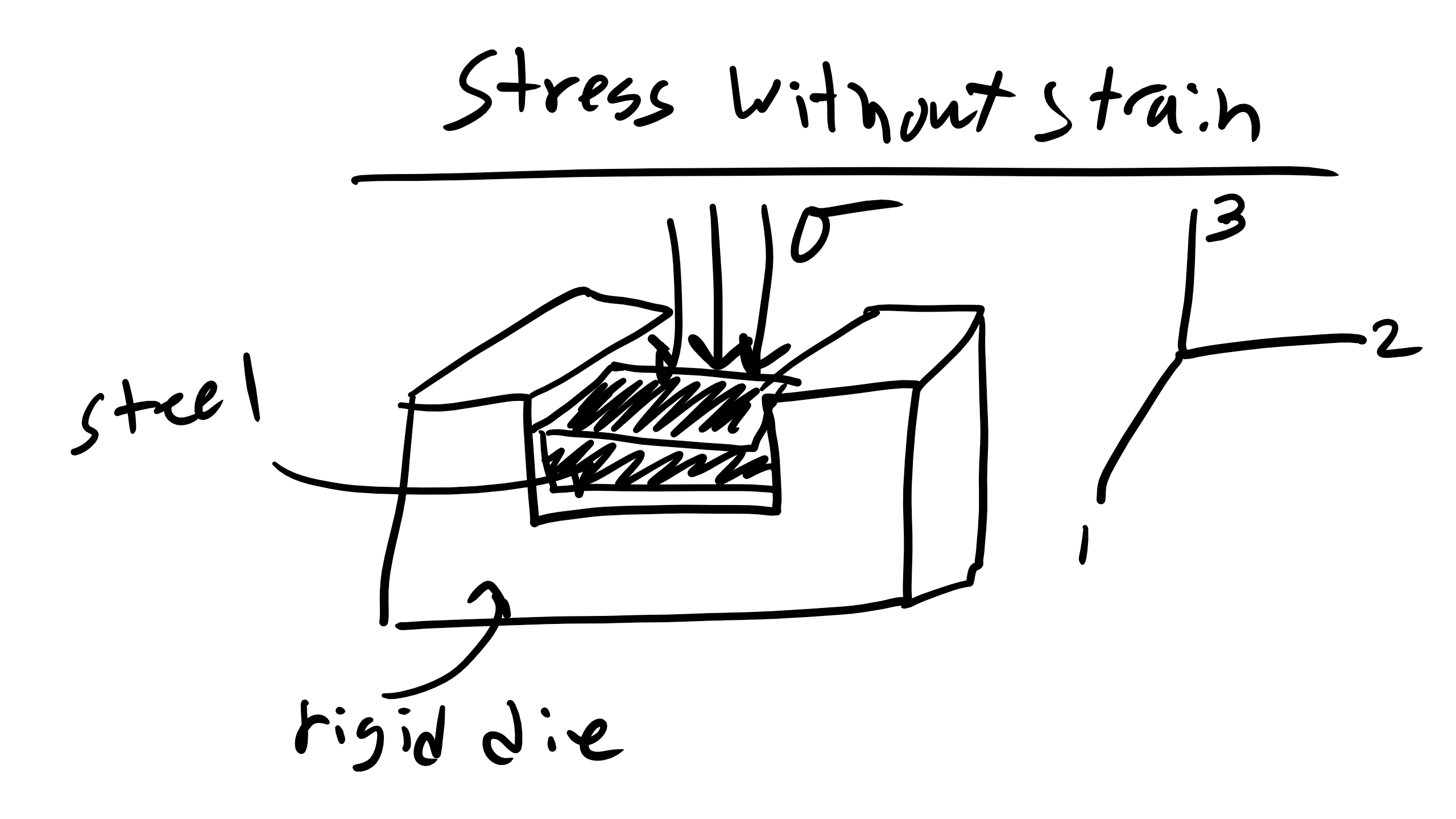
a.) State all the components of the stress tensor under the applied stress.
b.) Which normal strain components are zero and why?
c.) Use your answers in part a) and b) to express the relationship between the non-zero stresses in this system.
The solution to this problem can be seen in the video here:
5.8 Resolving Stress on Plane of Interest:
Now I know that all of you are statics experts so one way that we can resolve the stresses in a new coordinate system is by first applying our static equilibrium conditions for the forces in our new coordinate system. So first, we must define a new coordinate system that aligns with the plane of interest, i.e. we must rotate our old coordinate axes (x,y) to align with our new coordinate axes (\(x', y'\)).
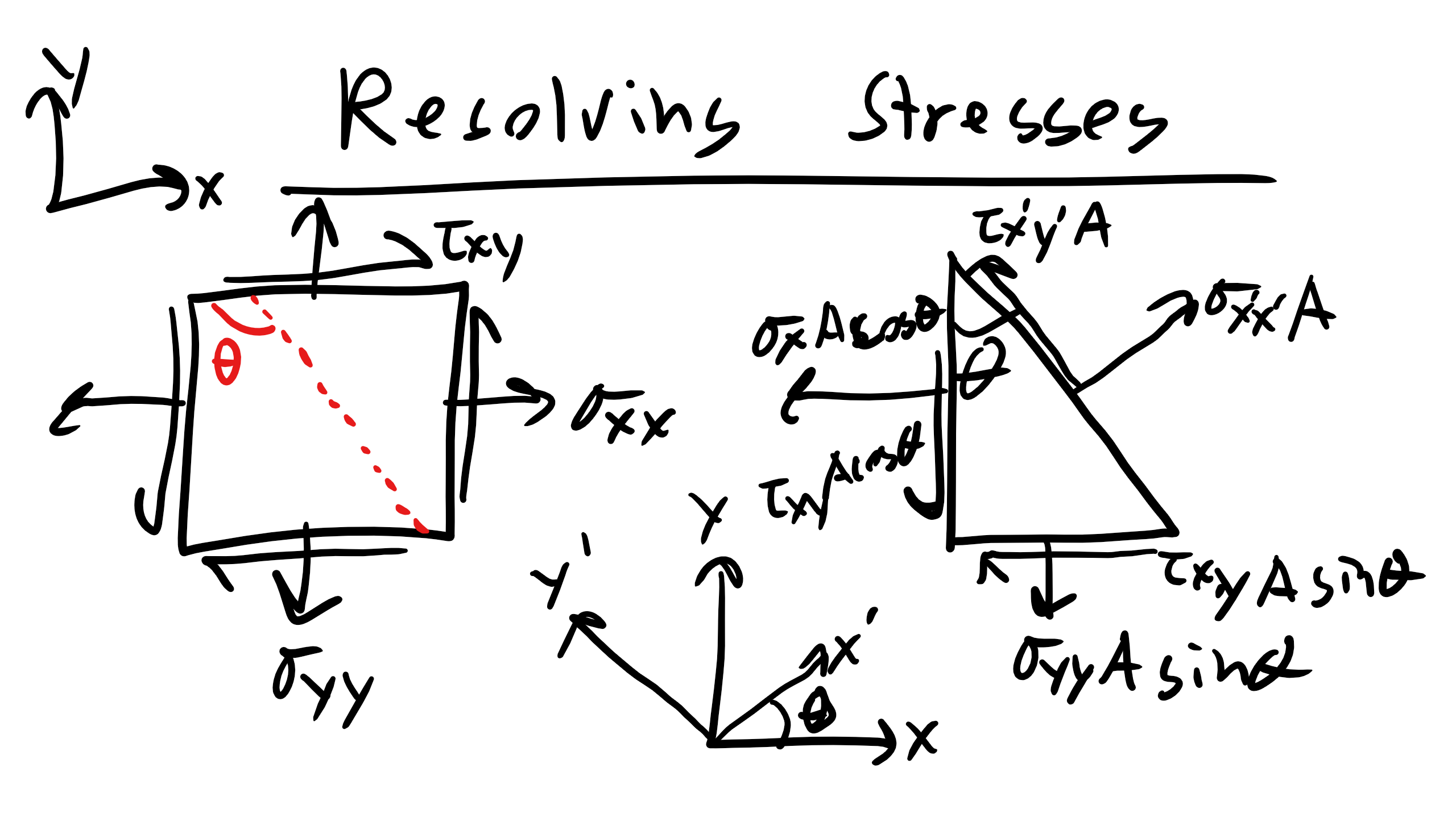
Then we balance out the forces assuming static equilibrium:
\begin{equation}
\sum F_{x'} = 0 = \sigma_{x'x'}A' - (\tau_{xy}A' \sin \theta) \cos \theta - (\sigma_{yy} A' \sin \theta) \sin \theta - (\tau_{xy} A' \cos \theta) \sin \theta - (\sigma_{xx} A' \cos \theta) \cos \theta
\end{equation}
After some rearranging and trig transformations:
\begin{equation}
\sigma_{x'x'}(\theta) = \frac{\sigma_{xx} + \sigma_{yy}}{2} + \frac{\sigma_{xx} - \sigma_{yy}}{2} \cos 2\theta + \tau_{xy} \sin 2 \theta
\label{eq1}
\end{equation}
\begin{equation}
\sigma_{y'y'}(\theta) = \frac{\sigma_{xx} + \sigma_{yy}}{2} - \frac{\sigma_{xx} - \sigma_{yy}}{2} \cos 2\theta - \tau_{xy} \sin 2 \theta
\label{eq2}
\end{equation}
\begin{equation}
\tau_{x'y'}(\theta) = - \bigg(\frac{\sigma_{xx}- \sigma_{yy}}{2}\bigg) \sin 2 \theta + \tau_{xy} \cos 2 \theta
\label{eq3}
\end{equation}
We have successfully transformed the stress state to our new coordinate system!
Now in addition to finding the stress state in a new coordinate system it is also helpful to find the principal stress state which is the stress state where there only exists normal stresses all shear stresses are equal to zero. To do this we can simply solve for when the normal stresses are maximized or when the shear stress values are zero and we will find that the principal stress angle will be simply
\begin{equation}
tan 2\theta = \frac{\tau_{xy}}{\frac{\sigma_{xx} - \sigma_{yy}}{2}}
\end{equation}
We can then substitute this back into the above equations and get:
\begin{equation}
\sigma_{1} = \frac{\sigma_{xx} + \sigma_{yy}}{2} + \sqrt{\bigg(\frac{\sigma_{xx} - \sigma_{yy}}{2}\bigg)^{2} + \tau_{xy}^{2}}
\end{equation}
\begin{equation}
\sigma_{2} = \frac{\sigma_{xx} + \sigma_{yy}}{2} - \sqrt{\bigg(\frac{\sigma_{xx} - \sigma_{yy}}{2}\bigg)^{2} + \tau_{xy}^{2}}
\end{equation}
\(\sigma_1\) and \(\sigma_2\) are the principal normal stresses and you can see by definition that \(\sigma_1\ > \sigma_2\). We can do the same for the maximum shear stress and find that
\begin{equation}
\tau_{xy,max} = \sqrt{\bigg(\frac{\sigma_{xx} - \sigma_{yy}}{2}\bigg)^{2} + \tau_{xy}^{2}}
\end{equation}
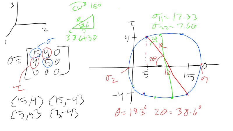
Now how many of you can do this upon request at a job interview or memorize these equations for 30+ years? My guess is probably not many of you can do so. Additionally, I like to refer this as the plug and chug method as it does not leave much intuition or thoughts students tend to just plug and chug into the equations. Plus I will tend to not ask questions that you can solve easily using these expressions so I would not utilize this method. Additionally, it is not general for the 3D stress state but let’s hold off on that for a while. But if we have the following stress-tensor below can we answer the questions below:
\begin{equation}
\sigma =
\begin{bmatrix}
15 & 4 & 0\\
4 & 5 & 0\\
0 & 0 &0 \\
\end{bmatrix}
\end{equation}
Now what is the principal stress state and the values of principal stress? What about the stress state 15o CW rotation around the 3 axis?
Now we can find this by plugging and chugging it into the equations we defined above.
However, this is not physical and we don’t really gain any intuition and most importantly it is a pain to do and when I ask harder questions this will be very difficult to do. But let's see how it is possible
5.8.1 Mohr’s Circle: A Graphical Approach
Another approach that is often the bane of many mechanics students is Mohr’s Circle. But today we will de-mystify Mohr’s circle and more importantly learn when it is useful to utilize this technique and when it is better and perhaps more appropriate to use our linear algebra approach.
Otto Mohr, a German engineer in the 1800’s, recognized that we can represent the principal stress state graphically. We can re-write the equations and
\begin{equation}
\bigg[\sigma_{1} - \bigg(\frac{\sigma_{xx} + \sigma_{yy}}{2}\bigg)\bigg]^{2} + \tau_{xy,max}^{2} = \bigg(\frac{\sigma_{xx} - \sigma_{yy}}{2}\bigg)^{2} + \tau_{xy}^{2}
\end{equation}
You should notice that this form has a similar form to the equation of a circle, i.e.
\begin{equation}
(x - c)^{2} + y^{2} = r^{2}
\end{equation}
where the center of the circle is \(\frac{\sigma_{xx} + \sigma_{yy}}{2}\) and the radius of the circle is \(\sqrt{(\frac{\sigma_{xx} - \sigma_{yy}}{2})^{2} + \tau_{xy}^{2}}\). We can plot Mohr’s circle for an arbitrary initial stress state.
The way that we will practically utilize Mohr’s circle is as follows, note that this works when considering plane stress states only
1. Draw a plot with normal stress on the x-axis and shear stress τ on the y-axis
2. Treat the stress tensor as a coordinate system with x-axis values for normal stress and y-axis values for shear stress. Plot the coordinates on the graph
3. The 4 coordinates that you may possible have (or 2 coordinates) are points that will lie on your Mohr’s circle. Draw a line connecting two of the points
4. When drawing the line pick the line such that the smaller normal stress has a positive shear stress value and the larger stress has the negative value, i.e. draw the top part of the line on the left and bottom on right.
5. Determine the length of this line as this will determine the diameter of your circle and thus the radius as well
6. Determine where the line crosses the x-axis this is the center of your Mohr’s circle.
7. Determine the angle between your line and the x-axis, this angle is 2\(\theta\). IT IS 2\(\theta\) DUE TO THE EQUATIONS AND TRANSFORMATIONS DESCRIBED ABOVE
8. Once you have the center, radius, and 2\(\theta\) values you can find the principal stress state, principal stress state angle, maximum shear stress value and angle, and then you can do geometry to get other stress states.
We can see this solved in the video here:
5.8.2 Plane Stress Linear Algebra Transformations
Now as we see above Mohr’s circle can be very useful for the geometrically gifted or inclined but I am not one of those people. Also, I find that when trying to determine the stress-state at an arbitrary rotation Mohr’s circle can become a bit cumbersome and I always fear that I may possible forget the 2\(\theta\) caveat.
So I would suggest instead or better yet to supplement Mohr’s circle we can use a linear algebra approach and a rotation matrix to convert stresses in one coordinate system to another coordinate system. Again, remember that we are still only working with plane stress states here, not 3D stress state transformations. So let’s get started.
Let’s start by first defining our transformation matrix T where
\begin{equation}
\begin{bmatrix}
T
\end{bmatrix}
=
\begin{bmatrix}
c^2 & s^2 & 2sc\\
s^2 & c^2 & -2sc\\
-sc & sc & c^2-s^2\\
\end{bmatrix}
\end{equation}
where \(c = \cos \theta \) and \(s = \sin \theta \).
So we now write that
\begin{equation}
\sigma^{'} = T \sigma
\end{equation}
or similarly
\begin{equation}
\begin{bmatrix}
\sigma_{11^{'}} \\
\sigma_{22^{'}} \\
\sigma_{12^{'}}
\end{bmatrix}
=
\begin{bmatrix}
c^2 & s^2 & 2sc\\
s^2 & c^2 & -2sc\\
-sc & sc & c^2-s^2\\
\end{bmatrix}
\begin{bmatrix}
\sigma_{11} \\
\sigma_{22} \\
\sigma_{12}
\end{bmatrix}
\end{equation}
So we can utilize this linear algebra approach and solve the same question but as you can see it is a very elegant way to solve these problems and requires minimal coding but you still have a clear intuition for how to solve these problems. However, often I will still draw the circle to keep the rotations clear. Here is the linear algebra approach solved here
5.8.4 Pressure Vessels: A Special Stress State
Finally let’s consider a very common scenario, a thin walled pressure vessel. The thin walled vessel has an applied pressure difference \(\Delta P\) between the internal pressure and the environment. The wall thickness is sufficiently small where we can say \(t << r\) or that \(\frac{r}{t}\) What is the stress state? It is plane stress state due to symmetry considerations. Therefore we need to find \(\sigma_1\) and \(\sigma_2\) which we will accomplish by drawing free body diagrams.

Let us first consider the longitudinal direction. Remember that the forces must sum to zero.
\begin{eqnarray}
\sum F_{1} = 0 = \Delta P \pi r^{2} - \sigma_{11} 2 \pi r t\\
\sigma_{11} = \sigma_{Longitudinal} = \frac{\Delta P r}{2 t}
\end{eqnarray}
We have the longitudinal stress so now let us look at the other direction, circumferential or hoop, and again the forces must sum to equal zero:
\begin{eqnarray}
\sum F_{2} = 0 = -\Delta P \Delta x 2 R + \sigma_{22} \Delta x t 2\\
\sigma_{22} = \sigma_{Hoop} = \frac{\Delta P R}{t}
\end{eqnarray}
As you can see the hoop stress is twice as large as the longitudinal stress so you should expect the material to fail in such a manner, unless there are extenuating conditions, i.e. defects, corrosion, different processing, etc. The strain ratio for hoop to longitudinal strain is nearly 4 : 1.
5.9 Beam Bending
Before we move into linear viscoelasticity, plasticity, fracture, and fatigue we have three elastic loading topics to discuss and these still very important and relevant loading states and phenomenon those being bending, buckling, and torsion respectively.
You have probably already encountered beam bending in other course and perhaps buckling but we again are going to take a slightly different approach specifically approaching this from the materials perspective.
Specifically we can define a beam as anything that can carry transverse loads and this can range from your typical civil engineering structural applications (bridges, trusses, pool diving boards, etc.) but also to some more exotic applications like Atomic Force Microscopy (AFM) which utilizes a cantilever beam, creating thin filmed substrate which have thermal mismatch which results in bending, cellular solids like foams, honeycomb structures, tissues, etc, sporting equipment like ski poles, and much much more!!
When dealing with beam bending problems we must consider several things before we start to approach the problem specifically we must consider
• Support Reactions
• Internal Forces
• Internal Moments
• Internal Stresses
• Deflections
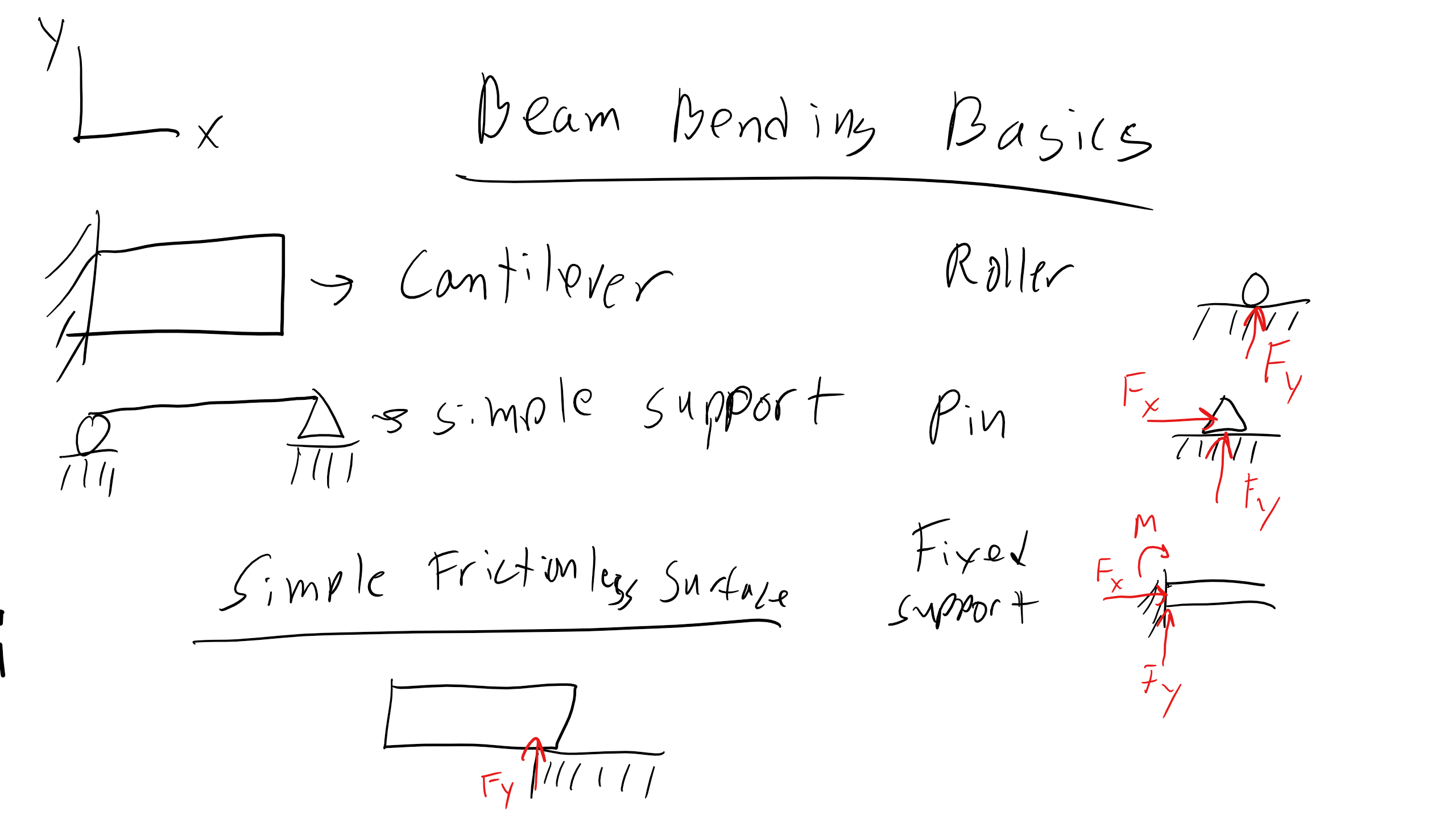
• Support Type: roller, pin, or fixed end
Additionally, different supports will have different reaction forces and moments for example
• Roller: Reaction force in the y-direction
• Pin: Reaction force in the x and y direction
• Simple Friction-less Surface: Reaction force in the y-direction
• Fixed Support: Reaction force in x, y, and reaction moment
Soon we will be working with free body diagrams as well as shear force and moment distributions within structures, now why do we want to do this? We need to find the locations of maximum shear forces and bending moments because material failure will often occur at regions of maximum shear forces which we will denote as V and bending moments M. These shear forces and bending moments can vary along the length of the beam. Moreover we will see that shear stress depends on the shear forces whereas normal stresses will depend on the bending moment. Finally the amount of deflection will also depend on the bending moment. Let’s start off with some background on how we will work with beams and support reaction diagrams, this should have been covered in other courses but let’s give us a nice little reminder.\
5.9.1 Sign Convention and Coordinate System Reminder Once Again
But again before we get started that let’s do one more reminder of our coordinate system and what we will determine as positive and negative forces, shears, moments, etc.
In terms of stresses tension will be defined as positive, compression as negative, shear is positive if the force is acting on a face with a normal in the positive direction and also has a force pointed in the positive direction.
For forces, forces which point in the positive direction relative to our coordinate system will be defined as positive. Also CCW moments are positive and CW moments are negative.
For beams a positive internal shear force V will be positive if it acts downward on the right hand face of a beam or upward on a left hand face of a beam. A positive internal bending moment M acts CCW on the right hand face of beam and CW on the left hand face of a beam. You can also consider a bending moment as positive if tension is on the bottom of the beam and negative if tension is at the top.

The key point to this entire discussion is before you approach any any any mechanics problem if there is not a coordinate system defined you must define one before you start anything. Keep this in mind it will be very important that you double check this as you approach problems.
5.9.2 Support Reactions in Beams
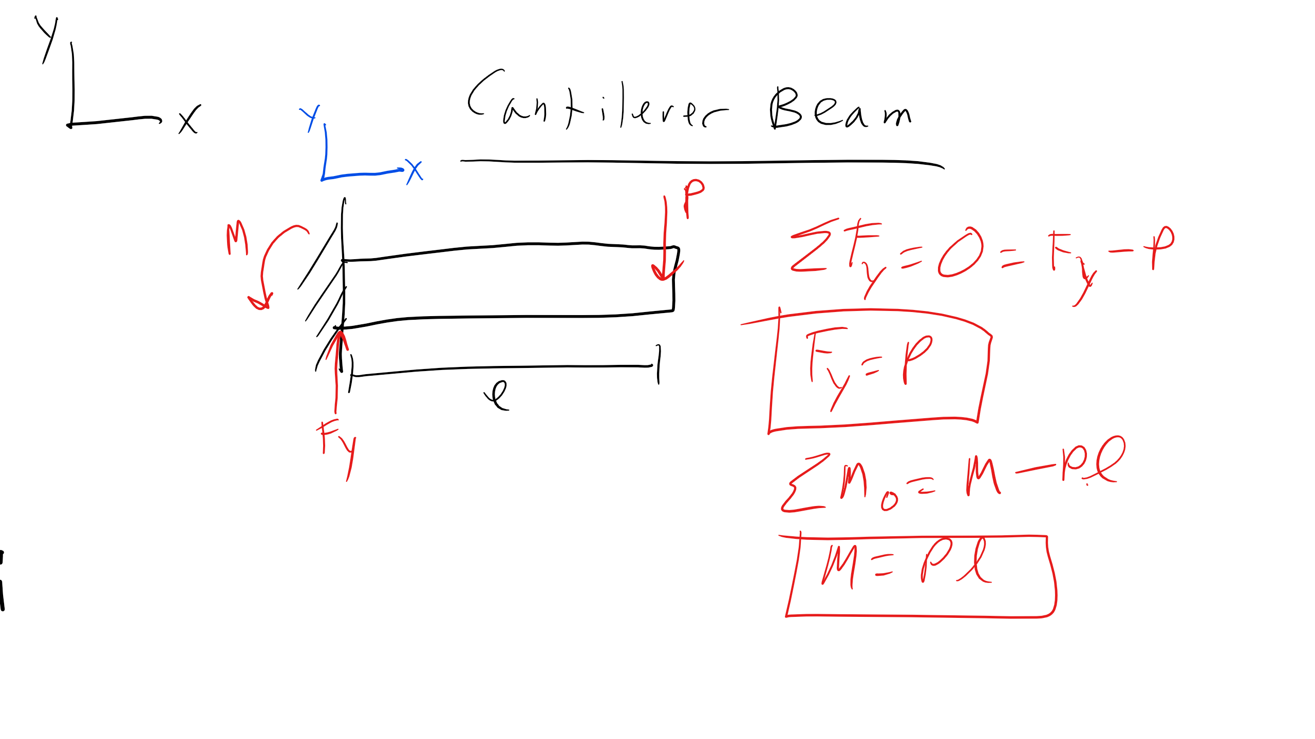
Let’s first consider a fixed end supported cantilever beam of length of length l with a load P applied at the end. At the fixed end we will have one reaction force Fy at the end.
For virtually all of our beam bending problems we will start as follows to develop our problem solving framework:
1. Coordinate System
2. Free Body Diagram
3. Equilibrium Expressions
4. Solve for Unknowns
As you can see below we have defined our coordinate system and we have drawn our free body diagram now we can apply our equilibrium conditions
\begin{eqnarray}
\Sigma F =0\\
\Sigma M =0
\end{eqnarray}
and solve for the reaction moment
\begin{eqnarray}
\Sigma F_y =0 = -P + F_{y}\\
\Sigma M_{0} = 0 = M_{0} -Pl\\
\end{eqnarray}
5.10 Stresses in Beams
Beam Bending Assumptions
So far we have demonstrated that when we apply a load on a beam internal shear and bending moments are created. This gives rise to both shear and normal stresses and typically as we will show the normal stress are much much greater than shear stresses, in particular when the length to height ratio of the beam is large, i.e. \(\frac{l}{h} > 10\). Again our entire purpose of learning about this topic is to avoid material failure so we will make sure to focus on regions of maximum stress. Now in doing so we will make several critical assumptions
• Beam is straight
• Material is linear elastic, isotropic, and cubic
• X-section is symmetric
• Beam is stable, i.e. no lateral buckling
Thus as the schematic below indicates typically we will be dealing with scenarios as we have done previously where one face is in tension and the other is in compression. There is also a plane along the longitudinal axis called the neutral axis that experiences no stress.
We must also distinguish between pure bending which exhibits a constant bending moment and non-uniform bending where the bending moment is not constant.
So typically when we bend a beam such that it experiences positive bending near the top the beam will be in compression and as we make our way to the bottom of the beam (height-wise) we will transition from compression to no stress at the neutral axis and then tension at the bottom of the beam. If the material is brittle failure will occur via crack propagation in the tensile regime whereas if a material is weak under compression failure will occur via buckling at the top surface. We have a good idea conceptually of what is going on but now we need to develop an expression that will tell us how this stress will be distributed in a beam. So let’s begin and we will derive this relationship in the following steps

1. Geometric Statement
2. Constitutive Equation
3. Equilibrium Conditions
So let’s start with our Geometric Statement
Geometric Statement
Let’s look at our schematic of our beam here and we can clearly see that sections \(\overline{mn}\) and \(\overline{pq}\) will rotate with respect to one another and if we extrapolate these lines that will intersect a particular point O which also the center of curvature. Additionally we can see that the distance from O to the neutral axis is given by the radius of curvature r. We will also assume that the distances between \(\overline{mn}\) and \(\overline{pq}\) at the neutral axis is constant dx so we can develop the following relationship such that our curvature \(\kappa\) is given by
\begin{equation}
\kappa = \frac{1}{\rho} = \frac{d\theta}{dx}
\end{equation}
and remember that if we have pure bending that \(\rho\) is constant and it will not be if we are in non-uniform bending. Additionally for curvature we have the same sense of positive and negative as the bending moment and as we have previously defined in other courses.
Constitutive Equation
We can now obtain that the normal strain in the x direction because we know that along all longitudinal planes other than the neutral axis will change length and produce strain in this direction. Let’s do a quick thought experiment and think about a segment \(\overline{ef}\) that is some distance y away from the neutral axis.

Here we find that
\begin{eqnarray}
l_o = dx = \rho d\theta\\
l_f = (\rho - y)d\theta\\
\epsilon_{xx} = \frac{l_f -l_o}{l_o} = -\frac{y}{\rho} = -y\kappa
\end{eqnarray}
Let’s look at this expression and that we see when the distance y approaches zero the strain also goes to 0 when we approach the neutral axis. Also when y is positive we have negative or compressive strain at the top of the beam and vice versa for the bottom all of which matches our intuition.
Now again we have been assuming that we are working in pure bending and that at the moment we are linear elastic isotropic and that we can neglect shear stresses because our beam is long so we can use Hooke’s law here but again be careful
\begin{equation}
\sigma_{xx} = E \epsilon_{xx} = -Ey\kappa
\end{equation}
so we see the stress varies linearly from the neutral axis. Additionally because we are dealing with simple uniaxial bending stress in the x direction we will also have the following strains \(\epsilon_{xx}, \epsilon_{yy}\), and \(\epsilon_{zz}\) which can be expressed as
\begin{eqnarray}
\epsilon_{xx} = -y\kappa\\
\epsilon_{yy} = \nu y\kappa \\
\epsilon_{zz} = \nu y\kappa \\
\end{eqnarray}
Equilibrium Conditions
We are almost done but now we have to apply our equilibrium conditions in order to relate our new fancy stress condition to the bending moment so let us first start with a differential element dA and we must find that the sum of all the forces in the x direction to be zero so we obtain
\begin{equation}
\Sigma F_x = 0 = \int_A \sigma_{xx} dA = \int_A -yE\kappa dA
\end{equation}
and since we know that both the curvature and Young’s modulus cannot be zero we will find that for our forces to sum to zero we must have that
\begin{equation}
\int_A y dA =0
\end{equation}
and remember from our previous discussion way back about the centroid and you will see that this is equivalent to saying that the centroid y must be equal to 0. So our z axis must pass through the centroid of the cross section and our neutral axis is in fact our z axis and thus our neutral axis must also pass through the centroid. Now all that is left is to take care of the moments and we find that if we consider the moment at our centroid or origin even though our force values sum to zero over the length of the beam there is a CW moment from our bending and that moment must be equivalent to the value of M(x) so we get the following relationship
\begin{equation}
\Sigma M_o = 0 = -M - \int_A \sigma_{xx} y dA
\end{equation}
and rearranging we get
\begin{equation}
M = - \int_A \sigma_{xx} y dA = E \kappa \int_A y^2 dA
\end{equation}
where we see that
\begin{equation}
I = \int_A y^2 dA
\end{equation}
where I is the moment of inertia and has units of m4. If we have a rectangular beam cross section as seen below we can calculate the moment of inertia.....
and we can obtain that
\begin{equation}
I_z = \int_A y^2 dA = \frac{bh^3}{12}
\end{equation}
We can do the same for for a circular cross section as well where J is the polar moment of inertia defined as
\begin{equation}
J = \int_A r^2 dA = \int_A (z^2+y^2) dA = 2I_z = \frac{\pi r^4}{4}
\end{equation}
Now with our definitions of moment of inertia clear we can now obtain our expression for the bending moment. Note that there are several cross-sections that are very good to resist bending based on the moment of inertia those being I-beams and honeycomb or cellular sandwich beams.
\begin{equation}
M = \kappa E I
\end{equation}
So we can now re-write our stress expression as a function of the bending moment as follows
\begin{equation}
\sigma_{xx} = - E \kappa y = -\frac{My}{I}
\end{equation}
Again we see that when the bending moment is positive and y is positive we have compression on the topic and vice versa for the bottom.
5.11 Beam Deflection
Thus far we have been focused almost exclusively on the forces, bending, and the stresses that develop in a beam when a load is applied. However, often it is extremely important to know who far a beam will deflect from the neutral axis. This is critical because certain materials or applications will have limitations on the amount of deflection which can occur. Additionally, we can also quite easily measure the amount of deflection and then back out the load or material properties as well.
Let’s take a look at a beam bending scenario below where we have some given amount of deflection v and there will also be some \(\Delta\) that describes the angle between the x axis and the tangent to the deflection curve. Now the question becomes what is the deflection at \(m_2\) in this scenario well we know that
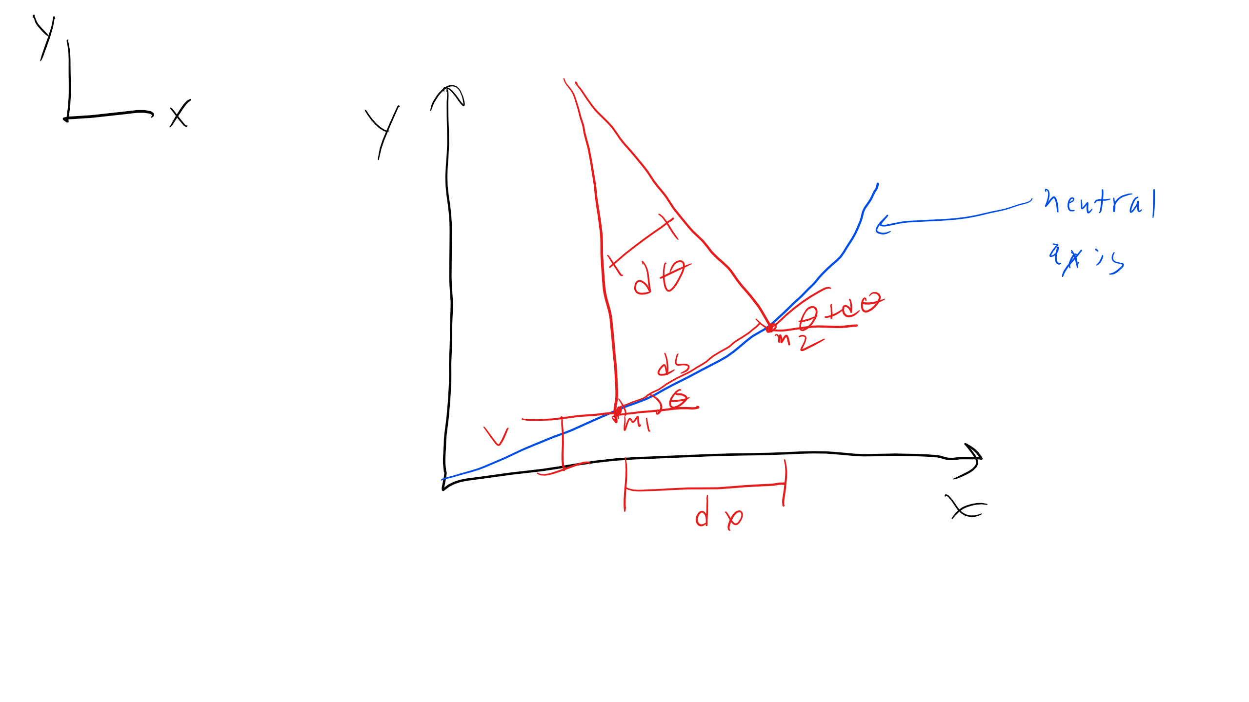
\begin{eqnarray}
\rho d\theta = ds\\
\kappa = \frac{1}{\rho} = \frac{d \theta}{ds}
\end{eqnarray}
We can also use the small angle approximation here such that for example
\begin{equation}
\cos \theta = \frac{dx}{ds} = 1
\end{equation}
therefore \(ds \approx dx\) so we can use this to obtain another expression for curvature such that
\begin{equation}
\kappa = \frac{d\theta}{ds} = \frac{d\theta}{dx} = \frac{d^2v}{dx^2}
\end{equation}
and we can also write the following very useful relationships
\begin{equation}
\frac{d\theta}{dx} = \frac{d^2 v}{dx^2} = \frac{M}{EI}
\end{equation}
This is a very useful relationship because we can integrate our M(x) twice to get the deflection and we can obtain the constants of integration by establishing boundary conditions. Additionally, this term EI is also referred to as the flexural rigidity which is very important for deflection
But we can develop an even more general equation for beam bending using the Euler-Bernouli equation which simply rearranges the equation we had above in terms of a general distributed load q as seen here
\begin{equation}
\frac{d^2}{dx^2}\bigg(\frac{E I dv^2}{dx^2}\bigg) = q
\end{equation}
and if we assume that the flexural rigidity is a constant we can simplify this equation as follows
\begin{equation}
EI \frac{d^4v}{dx^4} = q(x)
\end{equation}
We can relate this equation now to bending moments and shear moments respectively as follows
\begin{equation}
M = EI \frac{d^2v}{dx^2}
\end{equation}
\begin{equation}
V = \frac{d}{dx} \bigg(EI \frac{d^2v}{dx^2}\bigg)
\end{equation}
So we have a 4th order ODE that we will have to solve in order to find the equation for beam deflection so we need 4 total boundary conditions for these problems....time to use Mathematica!!
Here it is critical to observe that the bending moment is related the second derivative of the deflection, and the shear moment is related to the third derivative of the displacement, this will be critical as we determine our boundary conditions, speaking of which.....
5.11.1 Boundary Conditions for Beam Bending
Here we can see some common boundary conditions for common beam bending scenarios

Figure \(\PageIndex{17}\): Beam Bending Boundary Conditions
Here we can see some common boundary conditions. For a cantilever beam bending scenario at a fixed support there can be no deflection and thus there will be no slope at the fixed boundary. There will however be a shear moment and bending moment hear however.
At the free end of the beam with no force added there will be no bending or shear moment.
When we have simple supported beam we now see at the supports we will have no deflection however if there is a load applied there will be a change in slope at these locations. However, as there is no clamp here there will be no restoring moment so the moment will be zero at these supports.
5.11.2 Deflection for Simple End Loaded Cantilever Beam Fixed Support
So let’s look at the problem below here we can identify several boundary conditions.

So for a cantilever beam we know that at the wall the beam will not deflect and that the slope of deflection should also be zero so the boundary conditions here will be
\begin{eqnarray}
v(0)=0\\
v'(0)=0
\end{eqnarray}
We also know that at the we have a free end so we know that the bending moment must be zero here and that the shearing moment must also be zero so
\begin{eqnarray}
v''(l)=0\\
EIv'''(0)=P
\end{eqnarray}
So finally we will also have to input our expression for the load applied as a function of x and we can do that in mathematica.
3 Point Bending Test

What about a very common bending test a 3 point bending which can be seen below
We can see our boundary condition and our fundamental equation here.
Distributed Load
We can even do distributed loads as seen below

We can see our boundary condition and our fundamental equation here and plugging into Mathematica we can find our solution below here
Now all of this beam bending leads us to a very important phenomenon and material failure mode, that being buckling.
5.12 Buckling
When a materials is placed under compression the material will not typically fail via crack propagation as compressive stress does not assist in crack propagation, typically. Instead many materials under pure compressive stress will fail via buckling.
We will examine a particularly ubiquitous but important problem that being column buckling. A column is defined as a long slender member that is being loaded in compression and buckling is an instability phenomenon. Now when we mention stability we are referring to whether the system will return to it’s initial state when perturbed from this initial state. Stable systems will return to the initial state whereas unstable systems will not. You have most likely seen this illustrated in a physics course where a ball rolling down a hill is unstable but one at the bottom of the well is stable. There are also neutral and metastable systems as well but more on that in other courses.
Now you may imagine that if I have a column a longer column will buckle at lower applied loads and if I increase the cross sectional area it will increase applied load required for buckling. Also associated with this phenomenon of buckling will cause a change in shape, i.e. bending will occur.
Let’s develop a framework to describe buckling.
First, lets start off with an ideal column with pinned ends.
Ideal Column with Pinned Ends
No for an ideal column with pinned ends we have several assumptions that must be met which include
• Straight Beam
• Linear elastic material
• Load aligned with Column axis
As the column is the process of buckling will proceed in several states first elastic shortening. The column is stable at this stage and will compress linearly and elastically. As the applied load increases there will be some critical load where the become will become unstable and it will start to curve/bend and become unstable. What is this critically applied load? how does it relate to flexural modulus, beam length, and beam geometry? Well let’s figure this out!!!
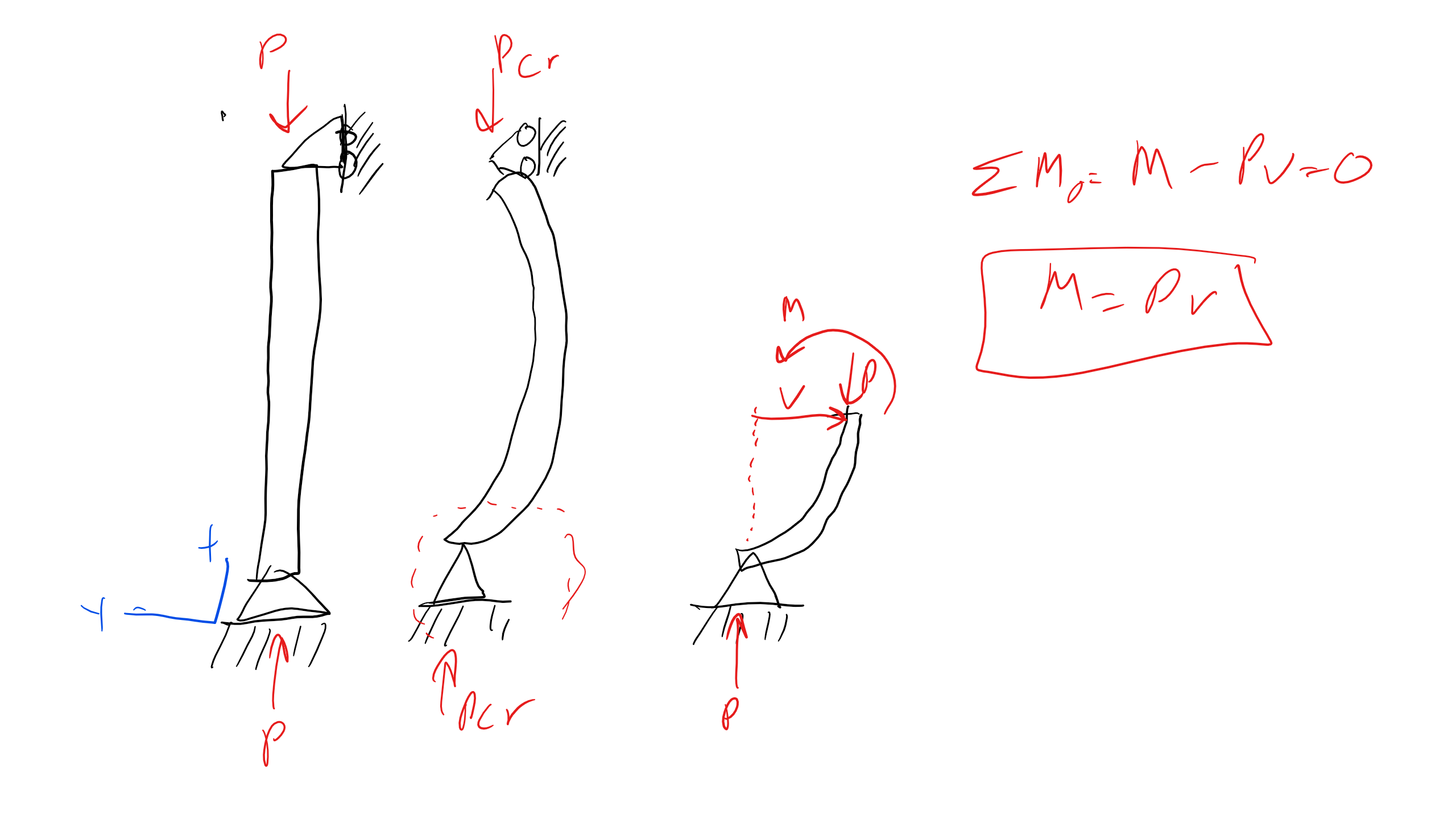
Let’s first start as usual by defining our coordinate system and drawing a free body diagram at the top of our beam and there will be some deflection v here
From the FBD we wee that the material will experience a bending moment M = Pv and we can relate this to our old friend
\begin{equation}
\frac{d^2v}{dx^2} = \frac{M}{EI} = \frac{Pv}{EI}
\end{equation}
with this differential equation we also have the following boundary conditions that
\begin{eqnarray}
v(0) = 0\\
v(l) = 0
\end{eqnarray}
We will get an expression in the form
\begin{equation}
v = c_1 \sin \sqrt{\frac{P}{EI}}x + c_2 \cos \sqrt{\frac{P}{EI}}x
\end{equation}
And thus we find that \(c_2 = 0\)but we also have a requirement that the sine term must go to zero so we have the following relationship that
\begin{equation}
\sqrt{\frac{P}{EI}}l = n \pi
\end{equation}
So the lowest value of loading that will lead to a deformed shape or buckling and thus the critical load for buckling is
\begin{equation}
P_{cr} = \frac{\pi^2 E I}{l^2}
\end{equation}
Now in terms of what n refers to physically it is the number of half-wavelengths along a column of length l. We see several interesting but expected phenomenon in this equation the first is that the critical load for buckling is linearly dependent on the flexural modulus but also scales as \(l^{-2}\)so the longer the beam the lower the critical load which makes sense intuitively. So if we Ideally we would also want a constant I about all cross sectional axes and to have the same buckling load about all axes.
5.13 Torsion
Torsion is a critical loading state and is extremely ubiquitous when it comes to the automotive industry. A twisting moment or torque are forces that act through a distance or a lever arm
\begin{equation}
T = r \times F
\end{equation}
where r is the vector representation of the lever arm and F is the force vector. Now when a material is under torsion the material experiences torsional stresses and displacements.
We can determine the torsional stresses and displacement using a very similar methodology as we did for the normal stresses and deflection in bending so we will follow our similar steps
1. Geometric Statement
2. Constitutive Equation
3. Equilibrium Conditions
Geometric Statement
Looking at our figure below we can defined some differential element dz which rotates some amount \(d\theta\) and so we can then relate the displacement \(\delta\) as follows

\begin{equation}
\delta = r d\theta
\end{equation}
Constitutive Equations
We know that this is very similar to our expression for shear strain so we can write that
\begin{equation}
\gamma_{z\theta} = \frac{\delta}{dz} = r\frac{d\theta}{dz}
\end{equation}
Additionally, assuming that we are in the linear elastic regime the shear stress is then given by
\begin{equation}
\sigma_{z\theta} = G\gamma_{z\theta} = Gr \frac{d\theta}{dz}
\end{equation}
Equilibrium Equations
Now we can apply our equilibrium conditions and here we will be concerned with summing the moments on a differential area dA and we can find that
\begin{equation}
T = \int_A \sigma_{z\theta} r dA = G \frac{d\theta}{dz} \int_A r^2 dA
\end{equation}
Also we have already found the expression for the moment of inertia for a hollow circular cross section as
\begin{equation}
I = \int^{r_o}_{r_i} r^2 2 \pi r dr = \frac{\pi (r^4_o - r^4_i}{2}
\end{equation}
We can also deal with part of the the expression below
\begin{eqnarray}
\frac{d\theta}{dz} = \frac{T}{GJ}\\
\theta = \int_z \frac{T}{JG} dz
\end{eqnarray}
![]()
where T, J, and G are constant in terms of z so we find that
\begin{equation}
\theta = \frac{Tl}{GJ}
\end{equation}
where the l is the length in the z direction.
Now we can finally plug back in to find that
\begin{equation}
\sigma_{z\theta} = G\gamma_{z\theta} = Gr \frac{d\theta}{dz} = \frac{Tr}{J}
\end{equation}
This is a very interesting expression because we see that these torsional stresses are independent of the choice of material because G has been removed form our expression.
This has a very nice analogy to our thin-walled pressure vessel expressions, there too we did not have any dependence on material selection but instead just on geometry.