
Chapter 4: Phase Diagrams
- Page ID
- 97982

\( \newcommand{\vecs}[1]{\overset { \scriptstyle \rightharpoonup} {\mathbf{#1}} } \)
\( \newcommand{\vecd}[1]{\overset{-\!-\!\rightharpoonup}{\vphantom{a}\smash {#1}}} \)
\( \newcommand{\dsum}{\displaystyle\sum\limits} \)
\( \newcommand{\dint}{\displaystyle\int\limits} \)
\( \newcommand{\dlim}{\displaystyle\lim\limits} \)
\( \newcommand{\id}{\mathrm{id}}\) \( \newcommand{\Span}{\mathrm{span}}\)
( \newcommand{\kernel}{\mathrm{null}\,}\) \( \newcommand{\range}{\mathrm{range}\,}\)
\( \newcommand{\RealPart}{\mathrm{Re}}\) \( \newcommand{\ImaginaryPart}{\mathrm{Im}}\)
\( \newcommand{\Argument}{\mathrm{Arg}}\) \( \newcommand{\norm}[1]{\| #1 \|}\)
\( \newcommand{\inner}[2]{\langle #1, #2 \rangle}\)
\( \newcommand{\Span}{\mathrm{span}}\)
\( \newcommand{\id}{\mathrm{id}}\)
\( \newcommand{\Span}{\mathrm{span}}\)
\( \newcommand{\kernel}{\mathrm{null}\,}\)
\( \newcommand{\range}{\mathrm{range}\,}\)
\( \newcommand{\RealPart}{\mathrm{Re}}\)
\( \newcommand{\ImaginaryPart}{\mathrm{Im}}\)
\( \newcommand{\Argument}{\mathrm{Arg}}\)
\( \newcommand{\norm}[1]{\| #1 \|}\)
\( \newcommand{\inner}[2]{\langle #1, #2 \rangle}\)
\( \newcommand{\Span}{\mathrm{span}}\) \( \newcommand{\AA}{\unicode[.8,0]{x212B}}\)
\( \newcommand{\vectorA}[1]{\vec{#1}} % arrow\)
\( \newcommand{\vectorAt}[1]{\vec{\text{#1}}} % arrow\)
\( \newcommand{\vectorB}[1]{\overset { \scriptstyle \rightharpoonup} {\mathbf{#1}} } \)
\( \newcommand{\vectorC}[1]{\textbf{#1}} \)
\( \newcommand{\vectorD}[1]{\overrightarrow{#1}} \)
\( \newcommand{\vectorDt}[1]{\overrightarrow{\text{#1}}} \)
\( \newcommand{\vectE}[1]{\overset{-\!-\!\rightharpoonup}{\vphantom{a}\smash{\mathbf {#1}}}} \)
\( \newcommand{\vecs}[1]{\overset { \scriptstyle \rightharpoonup} {\mathbf{#1}} } \)
\(\newcommand{\longvect}{\overrightarrow}\)
\( \newcommand{\vecd}[1]{\overset{-\!-\!\rightharpoonup}{\vphantom{a}\smash {#1}}} \)
\(\newcommand{\avec}{\mathbf a}\) \(\newcommand{\bvec}{\mathbf b}\) \(\newcommand{\cvec}{\mathbf c}\) \(\newcommand{\dvec}{\mathbf d}\) \(\newcommand{\dtil}{\widetilde{\mathbf d}}\) \(\newcommand{\evec}{\mathbf e}\) \(\newcommand{\fvec}{\mathbf f}\) \(\newcommand{\nvec}{\mathbf n}\) \(\newcommand{\pvec}{\mathbf p}\) \(\newcommand{\qvec}{\mathbf q}\) \(\newcommand{\svec}{\mathbf s}\) \(\newcommand{\tvec}{\mathbf t}\) \(\newcommand{\uvec}{\mathbf u}\) \(\newcommand{\vvec}{\mathbf v}\) \(\newcommand{\wvec}{\mathbf w}\) \(\newcommand{\xvec}{\mathbf x}\) \(\newcommand{\yvec}{\mathbf y}\) \(\newcommand{\zvec}{\mathbf z}\) \(\newcommand{\rvec}{\mathbf r}\) \(\newcommand{\mvec}{\mathbf m}\) \(\newcommand{\zerovec}{\mathbf 0}\) \(\newcommand{\onevec}{\mathbf 1}\) \(\newcommand{\real}{\mathbb R}\) \(\newcommand{\twovec}[2]{\left[\begin{array}{r}#1 \\ #2 \end{array}\right]}\) \(\newcommand{\ctwovec}[2]{\left[\begin{array}{c}#1 \\ #2 \end{array}\right]}\) \(\newcommand{\threevec}[3]{\left[\begin{array}{r}#1 \\ #2 \\ #3 \end{array}\right]}\) \(\newcommand{\cthreevec}[3]{\left[\begin{array}{c}#1 \\ #2 \\ #3 \end{array}\right]}\) \(\newcommand{\fourvec}[4]{\left[\begin{array}{r}#1 \\ #2 \\ #3 \\ #4 \end{array}\right]}\) \(\newcommand{\cfourvec}[4]{\left[\begin{array}{c}#1 \\ #2 \\ #3 \\ #4 \end{array}\right]}\) \(\newcommand{\fivevec}[5]{\left[\begin{array}{r}#1 \\ #2 \\ #3 \\ #4 \\ #5 \\ \end{array}\right]}\) \(\newcommand{\cfivevec}[5]{\left[\begin{array}{c}#1 \\ #2 \\ #3 \\ #4 \\ #5 \\ \end{array}\right]}\) \(\newcommand{\mattwo}[4]{\left[\begin{array}{rr}#1 \amp #2 \\ #3 \amp #4 \\ \end{array}\right]}\) \(\newcommand{\laspan}[1]{\text{Span}\{#1\}}\) \(\newcommand{\bcal}{\cal B}\) \(\newcommand{\ccal}{\cal C}\) \(\newcommand{\scal}{\cal S}\) \(\newcommand{\wcal}{\cal W}\) \(\newcommand{\ecal}{\cal E}\) \(\newcommand{\coords}[2]{\left\{#1\right\}_{#2}}\) \(\newcommand{\gray}[1]{\color{gray}{#1}}\) \(\newcommand{\lgray}[1]{\color{lightgray}{#1}}\) \(\newcommand{\rank}{\operatorname{rank}}\) \(\newcommand{\row}{\text{Row}}\) \(\newcommand{\col}{\text{Col}}\) \(\renewcommand{\row}{\text{Row}}\) \(\newcommand{\nul}{\text{Nul}}\) \(\newcommand{\var}{\text{Var}}\) \(\newcommand{\corr}{\text{corr}}\) \(\newcommand{\len}[1]{\left|#1\right|}\) \(\newcommand{\bbar}{\overline{\bvec}}\) \(\newcommand{\bhat}{\widehat{\bvec}}\) \(\newcommand{\bperp}{\bvec^\perp}\) \(\newcommand{\xhat}{\widehat{\xvec}}\) \(\newcommand{\vhat}{\widehat{\vvec}}\) \(\newcommand{\uhat}{\widehat{\uvec}}\) \(\newcommand{\what}{\widehat{\wvec}}\) \(\newcommand{\Sighat}{\widehat{\Sigma}}\) \(\newcommand{\lt}{<}\) \(\newcommand{\gt}{>}\) \(\newcommand{\amp}{&}\) \(\definecolor{fillinmathshade}{gray}{0.9}\)4.1 Lowest Energy Wins!
I have recorded a series of lectures to supplement the text which can be found in the playlist below:
https://www.youtube.com/playlist?lis...1CCqf55NMUHETA
Materials can exist as different phases, i.e. solid, liquid, gas, vapor, plasma and each of those phases are described by their own unique free energy curve. The thermodynamically stable phase is the one with the lowest free energy at any given temperature, pressure, composition, etc. And crossing points in the free energy curves will define the locations of phase transitions. We can see this schematically when considering a pure single component material going undergoing melting and we can plot the free energy as function of temperature and see the phase transition.

![]()
where \(G_l\) is the molar Gibbs free energy of the liquid phase and \(G_s\) is the molar Gibbs free energy of the solid phase. I will try to be as consistent as possible to keep liquid as blue color, like water.
We can also draw this out for the complete phase transition spectrum for a given material as the solid melts, the liquid boils, and the solid can sublimate directly to vapor.

However as we touched upon in structure materials can exhibit different crystalline forms in the solid state depending on the conditions of temperature and pressure.
What was the special name for these materials?
Polymorphs/allotropes.
Wouldn’t it be useful to have some type of diagram that would allow us to visualize these different phases....hmmm....!
4.2 Phase Diagrams of Single-Component Materials
Phase diagrams illustrate the phases of a system at equilibrium as a function of 2 or more thermodynamic variables.
Phase diagrams are also particularly useful because they obey the laws of thermodynamics and there are constraints on the structure of phase diagrams, particularly the Gibbs Phase Rule.
4.3 Gibbs Phase Rule
The Gibbs Phase Rule determines how many phases can be in equilibrium simultaneously and when those phases are stable along a field, line, or point in the phase diagram. There are two criteria for phase equilibrium at a constant temperature and pressure are that the chemical potential of each component must be equal in each phase:
\begin{eqnarray}
\mu^{\alpha}_{1}=\mu^{\beta}_{1}=\mu^{\gamma}_{1}=\mu^{P}_{1}...\\
\mu^{\alpha}_{2}=\mu^{\beta}_{2}=\mu^{\gamma}_{2}=\mu^{P}_{2}...\\
\mu^{\alpha}_{C}=\mu^{\beta}_{C}=\mu^{\gamma}_{C}=\mu^{P}_{C}...
\end{eqnarray}
So we end up with C(P-1) equations. And we also have the second condition which is given by the Gibbs-Duhem equation
\begin{eqnarray}
V^{\alpha}dP - S^{\alpha}dT - \sum_{i=1}^{c} n^{\alpha}_{i}d\mu^{\alpha}_{i}=0\\
V^{\beta}dP - S^{\beta}dT - \sum_{i=1}^{c} n^{\beta}_{i}d\mu^{\beta}_{i}=0\\
V^{\gamma}dP - S^{\gamma}dT - \sum_{i=1}^{c} n^{\gamma}_{i}d\mu^{\gamma}_{i}=0
\end{eqnarray}
So here we end up with P equations. So the degrees of freedom (DOF) is total number of variables - the total number of equations.
\begin{eqnarray}
D = (CP +2) - (C(P-1) +P)\\
D = C - P + 2
\end{eqnarray}
where D is the degrees of freedom, C is the number of components, P is the number of phases. The 2 comes from T and P as independent variables.
So let’s do a couple of examples where we apply the Gibbs phase rule! Let’s look at the single-component phase diagram below:

What is the DOF for the 1st X location?
The DOF is 2.
\begin{eqnarray}
D + P = C + 2\\
D +1 = 1 + 2
\end{eqnarray}
That means we can vary both T and P and still be in the liquid phase.
What is the DOF for the 2nd X location?
The DOF is 1. We can now only vary T or P freely the other is fixed.
What is the DOF for the 3rd X location?
The DOF is 0. We can not move anywhere. This is an invariant or triple point.
Now there is one unique point, an invariant point, called the triple point that can allow the 3 phases to co-exist, i.e. any change in the variables will cause the equilibrium to shift to either 1 or 2 phases in equilibrium. The slope of the 2-phase line on the P vs. T diagram is determined by the Clausius-Clapeyron equation evaluated at the coexistence curve:
\begin{equation}
\frac{dP}{dT} = \frac{\Delta \overline{S}^{S \rightarrow L}}{\Delta \overline{ V}^{S \rightarrow L}} = \frac{\Delta \overline{S}_{m}}{\Delta \overline{V}_{m}} =\frac{\Delta \overline{H}_{m}}{T_{m} \Delta\overline{ V}_{m}}
\end{equation}
We know that typically the enthalpy of melting is positive so the slope of the P-T diagram for the solid-liquid coexistence curve should be positive. Let’s look at iron on the lecture slides.
4.4 Multi-Component Phase Diagrams
So far we have only dealt with phase diagrams of pure components but typically you will deal with either binary, ternary, quaternary, etc. phase diagrams.
Let’s take a look at a relatively simple phase diagram, a Binary Lens phase diagram which holds for ideal solution scenarios.
(Side Note: When I say something is simple please do not interpret this as the concept being easy. These concepts are very difficult but what I mean by the problem is simple I want to encourage and show you that all these problems can be solved. When we say that this or that problem is really difficulty that problem is a given a special mystique and students might be wary about going about soling the problem or learning that concepts. By saying something is simple I want to remove that mystique.)
Note here that we are not varying pressure now because typically we are working in a constant pressure environment, although that is not necessarily always the case. Now this will change our Gibbs phase rule condition to:
\begin{equation}
\mu = \bigg (\frac{\partial G}{\partial n}\bigg)_{T,P}
\end{equation}
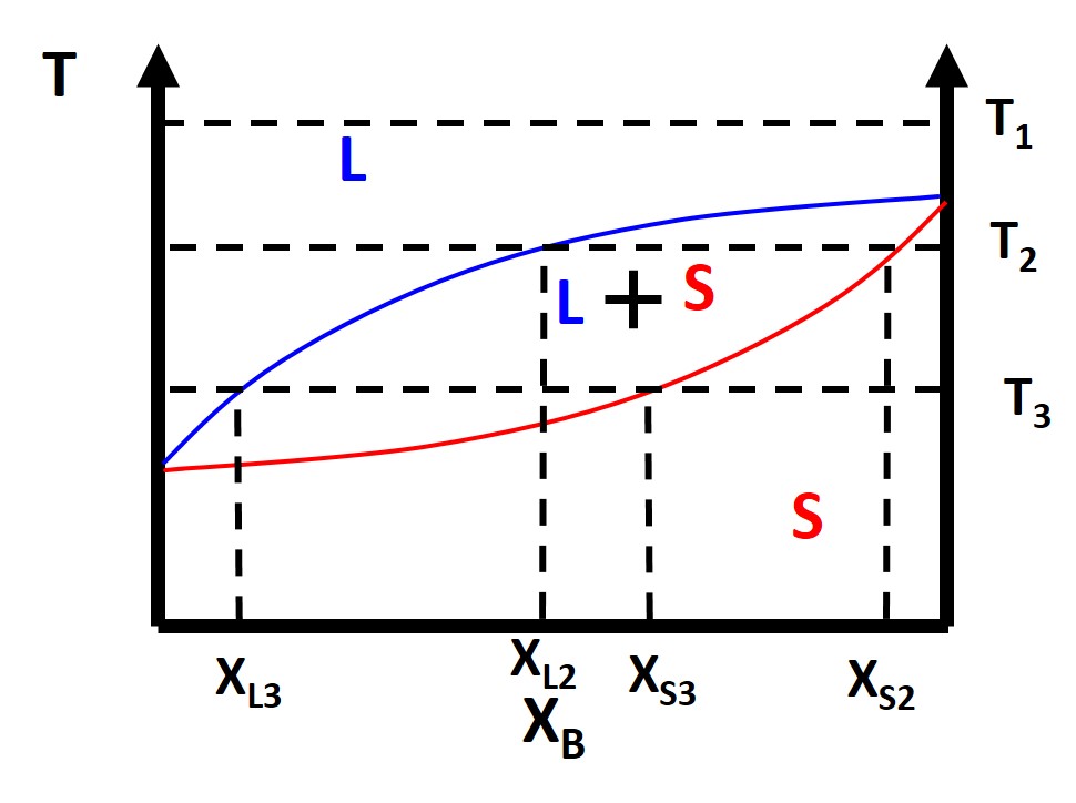
Figure \(\PageIndex{4}\): Binary Lens Phase Diagram
We can also take a look at the free energy diagrams as well to conceptualize the phase diagrams. At \(T_1\) everything is as usual in terms of our free energy diagram with liquid phase being lower energy than the solid phase. Things start to get a little funky at where we have the two phase region of a solid and liquid. What happens here? Why does this occur? Well at compositions less than \(X_{L2}\) and greater than \(X_{S2}\) everything is normal. What happens is in between these compositions. You see that we can draw a common tangent line (purple). When you have a common tangent line the system can phase separate from a 1-component system (liquid) to a weighted mixture of two components (solid and liquid) which has a lower free energy than the starting 1-component phase. This is because the requirement for equilibrium as we previously mentioned is that the chemical potential of each component must be equal in all phases and we have the expression that the chemical potential \(\mu\) is
\begin{equation}
\bigg (\frac{\partial G}{\partial X}\bigg)_{X = X^\alpha} = \bigg (\frac{\partial G}{\partial X}\bigg)_{X = X^\beta}
\end{equation}
So common tangent rule will allow us to find your equilibrium volume fraction of species in each phase via the common tangents in free energy curves and the slope is essential the chemical potential so when the slope is equal. So between the common tangent points equilibrium will have the components in both phases, i.e. mixed as given below

4.5 The Lever Rule:
Typically we are also interested in finding at a particular composition and temperature what will be the relative fractions of the different phases of the material, or in the case of a simple lens diagram, what fractions will be solid and liquid. To calculate these phase fractions we will use the lever rule. Once you pick a temperature of interest, \(T_1\), and a composition, \(X^o_B\) then you draw a horizontal isotherm which connects or ties together the boundaries of a two phase regions. These horizontal isotherms are also called tie lines.
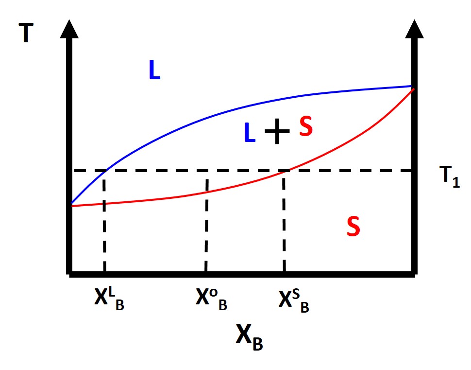
The composition of the liquid and solid phases, \(X^L_B\) and \(X^S_B\), respectively are simply where the tie line intersects the liquidus or solidus lines, again respectively. The liquids line defines the two phase coexistence between a liquid and a solid phase. The solidus line represent the two phase coexistence between a solid and another solid phase, for binary phase diagrams. We can also calculate the fraction of phases that are present by using the lever rule. What you do is simply take the length of the tie line from the composition, \(X^o_B\) , to the phase boundary for the other phase and divide by the total tie line length. For example:
\begin{eqnarray}
f^{S} = \frac{X^{o}_{B}-X^{L}_{B}}{X^{S}_{B}-X^{L}_{B}}\\
f^{L} = \frac{X^{S}_{B}-X^{o}_{B}}{X^{S}_{B}-X^{L}_{B}}
\end{eqnarray}
where \(f^S\) and \(f^L\) are the phase fractions of solid and liquid respectively. This is typically the simplest type of phase diagram that you will find and it is actually the phase diagram for Cu-Ni. This also hold for ideal solution scenarios but typically most binary solutions or alloys will not be miscible at all compositions and temperatures. We know from structure that different materials have different crystal structures so those crystal structures might not always be compatible.
4.6 Phase Transitions Congruent vs Incongruent
A phase transition can occur congruently or incongruently. A congruent phase transition occurs when there is a complete transformation from one phase to another with no change in composition as seen in the examples below. An incongruent phase transition is a partial transformation from one phase to another and there will be a change in composition like we just saw with the lens diagram.
4.7 Eutectic Phase Diagram
So far we have only discussed the simple binary lens phase diagram which only applied to several real experimental systems. There is another relatively simple phase diagram that corresponds to many more experimental systems and that is the binary eutectic phase diagram.
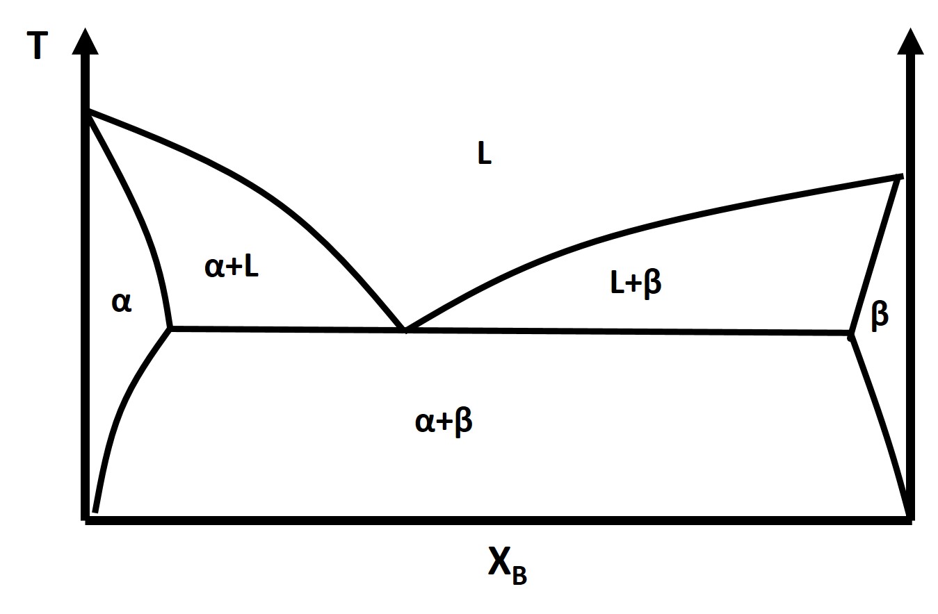
The binary eutectic phase diagram has several distinctive features one being a solid-solid phase mixture, limit of solubility at different temperatures, and an invariant point in the phase diagram, the eutectic point.
The solubility limit is the maximum amount of solute that you can integrate into the structure (or phase) or the solvent to form a solid solution. The solubility limit is a function of temperature and must be defined at a given temperature.
What is the solubility limit of B into A at \(T_1\)?
What about A into B?
Identify the Solidus Line
The eutectic point is an invariant point, D = 0, and it describes the constant composition transformation from a pure liquid phase to a two phase solid solution/mixture or alternatively
\begin{equation}
L \rightleftarrows \alpha + \beta
\end{equation}
There are also a number of different invariant points beyond the simple eutectic.
4.8 Eutectic, Eutectoid, Peritectic, Peritectoid, and Monotectic
We have already discussed one invariant point, the eutectic. There is also another invariant point called the eutectoid. The eutectoid describes the constant composition transformation from a pure solid phase to two phase solid solution/mixture as described below
\begin{equation}
\gamma \rightleftarrows \alpha + \beta
\end{equation}
There is also a peritectic invariant point. The peritectic describes where a solid and liquid phase mixture will transform into a pure solid phase which is described by the equation below
\begin{equation}
L +\alpha \rightleftarrows \beta
\end{equation}
Finally the last invariant point is described by the peritectoid which is a transformation of two solid phases in a mixture to a single solid phase again described by the equation below
\begin{equation}
\gamma + \alpha \rightleftarrows \beta
\end{equation}
There is also a monotectic invariant point that does not appear in to many phase diagrams but this invariant point describes the transformation from a pure liquid to another liquid and solid phase which is described by the equation below:
\begin{equation}
L_{1} \rightleftarrows L_{2} + \alpha
\end{equation}
Let’s do a couple of examples were we identify the invariant points in a couple of phase diagrams and calculate the fraction of phases at a given composition and temperature.
4.8.2 Ternary and Quaternary Phase Diagrams
So far we have dealt with relatively simple binary phase diagrams however there are also much more complicated ternary and quaternary phase diagrams. These types of phase diagrams are crucial, particularly in the field of ceramics. We can perform the same type of analysis on these diagrams but of course it becomes more complex.
4.9 Stable vs. Metastable Phase Boundaries: Cahn-Hilliard Spinodal Decomposition
We just touched upon the concept of stability and metastable with martensite. So let us define the conditions for stability. For a closed system at constant temperature and pressure the Gibbs free energy is minimized with respect to fluctuations in other extensive variables, particularly fluctuations in composition. To be stable against these fluctuations we have an additional condition on the second derivative of the free energy which is given by Le Chatelier’s principle: A system perturbed by a small fluctuation will elicit a thermodynamic driving force to return to the stable equilibrium state . Or in terms of fluctuations in composition the condition for stability is
\begin{equation}
\frac{\partial^{2}G}{\partial X^{2}_{B}} > 0
\end{equation}
Let’s take a look at this condition in the graph below
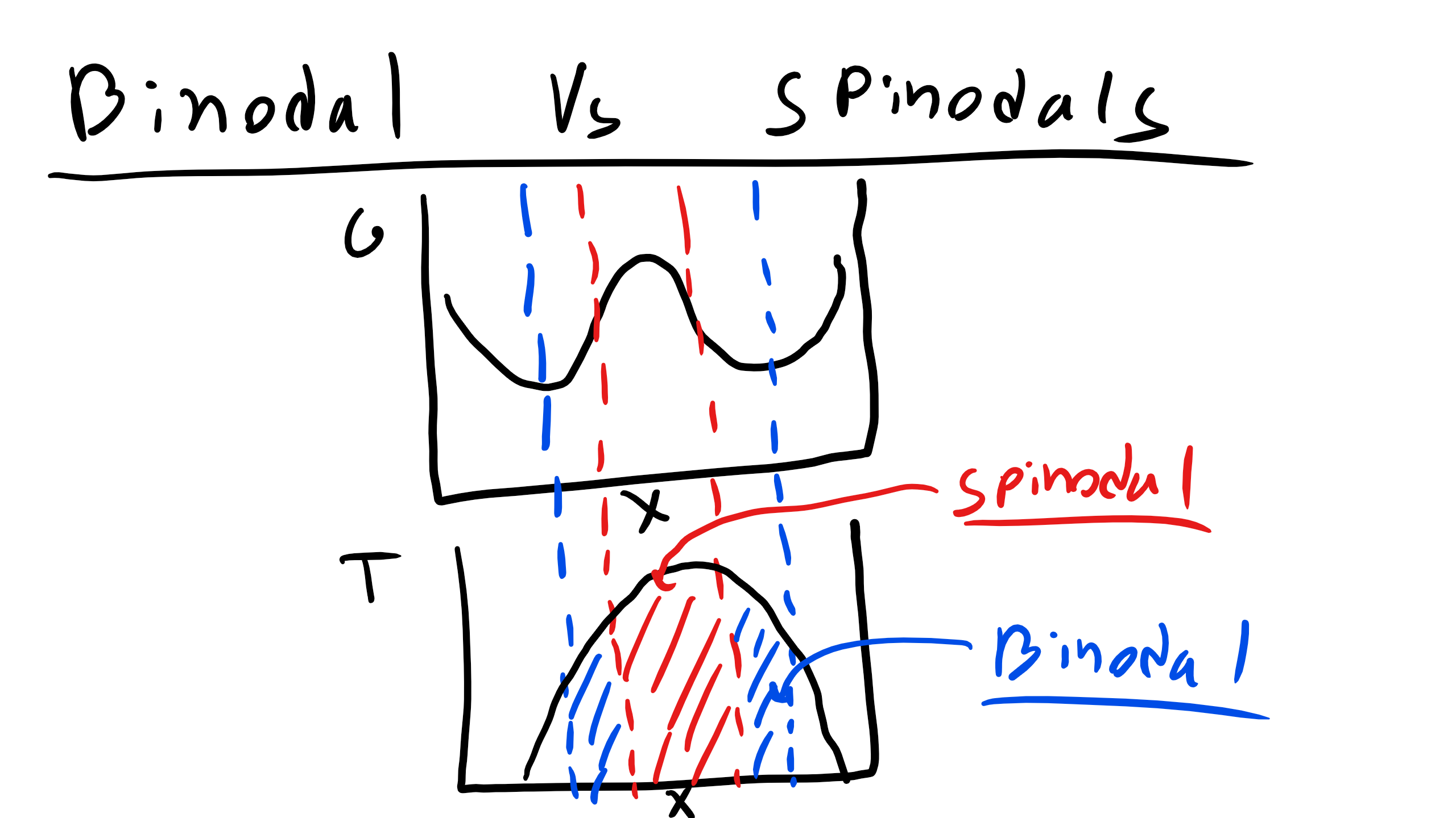
We can clearly see here that we have several special points binodals and spinodals.
Binodals are defined by the following mathematical relations
\begin{eqnarray}
\frac{\partial G}{\partial X_{B}} =0\\
\frac{\partial^{2}G}{\partial X^{2}_{B}} > 0
\end{eqnarray}
while spinodals are defined by
\begin{equation}
\frac{\partial^{2}G}{\partial X^{2}_{B}} = 0
\end{equation}
We can also see a point in this diagram that is unstable where
\begin{eqnarray}
\frac{\partial G}{\partial X_{B}} =0\\
\frac{\partial^{2}G}{\partial X^{2}_{B}} < 0
\end{eqnarray}
The spinodal points will define the spinodal boundary and the binodal points will define the boundaries of the 2-phase regions. Systems that are initially unstable will undergo spinodal decomposition while systems that are initially stable or metastable will evolve via nucleation and mechanisms. Spinodal decomposition is a homogeneous transformation while nucleation and growth is typically dominated by a heterogeneous process.
4.10 First Order vs Second Order Phase Transitions
This discussion brings us nicely to a discussion on the order of phase transformations. So far we have really been focused on first order phase transformations like a crystal melting, water boiling, allotropes, etc, these are all first order phase transformations.
Why is that?
Well when we discuss order we are talking about whether the transformation is accompanied by a discontinuity in a first, second, or higher order derivative of Gibbs free energy.
The second order transitions are also called continuous phase transitions because the first derivative of Gibbs is continuous and it is not until there is a second order derivative that a discontinuity is observed. Some examples of second order transitions are ODT (Order Disorder Transitions), glass transitions, superconducting transitions, ferromagnetic to paramagnetic transitions.
We can see how these transitions look like by looking at Gibbs free energy.

Remember from thermo that:
\begin{eqnarray}
S = -\bigg(\frac{\partial G}{\partial T}\bigg)_{P,n}\\
C_{p} = -T\bigg(\frac{\partial^{2} G}{\partial T^{2}}\bigg)_{P,n}
\end{eqnarray}