10.3: Phasor and Complex Numbers

Introduction

In engineering and applied science, three test signals form the basis for our study of electrical and mechanical systems. The impulse is an idealized signal that models very short excitations (like current pulses, hammer blows, pile drives, and light flashes). The step is an idealized signal that models excitations that are switched on and stay on (like current in a relay that closes or a transistor that switches). The sinusoid is an idealized signal that models excitations that oscillate with a regular frequency (like AC power, AM radio, pure musical tones, and harmonic vibrations). All three signals are used in the laboratory to design and analyze electrical and mechanical circuits, control systems, radio antennas, and the like. The sinusoidal signal is particularly important because it may be used to determine the frequency selectivity of a circuit (like a superheterodyne radio receiver) to excitations of different frequencies. For this reason, every manufacturer of electronics test equipment builds sinusoidal oscillators that may be swept through many octaves of Orequency. (Hewlett-Packard was started in 1940 with the famous HP audio oscillator.)

In this chapter we use what we have learned about complex numbers and the function \(e^{jθ}\) to develop a phasor calculus for representing and manipulating sinusoids. This calculus operates very much like the calculus we created in "Complex Numbers" and "The Functions e^x and e^jθ" for manipulating complex numbers. We will apply these mathematical representations to the study of AC circuits.

To begin, we want to consider a transmission line that being excited with an oscillating source, as in Figure \(\PageIndex{1}\).

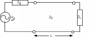Figure \(\PageIndex{1}\): Sinusoidal excitation of a loaded transmission line

The usual set-up includes a source, with a sinusoidal output, a source impedance \(Z_{g}\), a transmission line with impedance \(Z_{0}\), length \(L\) meters, and a load of impedance \(Z_{L}\) at the end.

Let's look at the source first. We can describe the output waveform from the generator as \[V(t) = V_{g} \cos (\omega t + \theta)\]

When plotted, this looks like Figure \(\PageIndex{2}\).

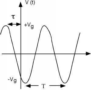Figure \(\PageIndex{2}\): Excitation waveform

The oscillating waveform has a period \(T\) and its angular frequency \(\omega\) is given as \[\begin{array}{l} \omega &=& \dfrac{2 \pi}{T} \\ &=& 2 \pi f \end{array}\]

The angle \(\theta\), which specifies how much the wave is leading a cosine function with zero off-set, is given by \[\theta = 2 \pi \frac{\tau}{T}\]

What we do not want to do is carry a bunch of sine and cosine functions around with us everywhere. Once we start multiplying and dividing, the trig turns into a big mess, and gets in the way of our understanding of what is going on. The way we deal with this is to introduce phasors.

Since we know from Euler's Identity \[V_{g} e^{i(\omega t + \theta)} = V_{g} (\cos (\omega t + \theta) + i \sin (\omega t + \theta)) = V_{g}\angle{\theta}\]

if we take a real part of \(V_{g} e^{i (\omega t + \theta)}\), we will extract the voltage waveform we desire. We will re-write this function as \[V_{g} e^{i (\omega t + \theta)} = V_{g} e^{i \omega} e^{i \omega t}\]

and then define \(\tilde{V}_{g}\) as the phasor voltage where \[\tilde{V}_{g} = V_{g} e^{i \theta}\]

Note that \(\tilde{V}_{g}\) is a complex quantity, with both a magnitude \(\left| V_{g} \right|\) and a phase angle \(\theta\). In order to retrieve a real voltage signal from a phasor, we have to multiply the phasor by \(e^{i \omega t}\) and then take the real part. Note that this is the same thing as plotting the phasor on the complex plane, and then observing the projection of the phasor on the real axis, as the phasor rotates around at a rate \(\omega t\) as shown in Figure \(\PageIndex{3}\).

Figure \(\PageIndex{3}\): Phasor representation

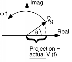
This method of visualization will sometimes help make results seem a little easier to understand, or at least check for reasonableness.

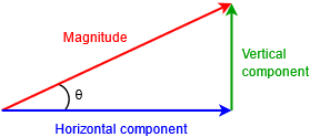
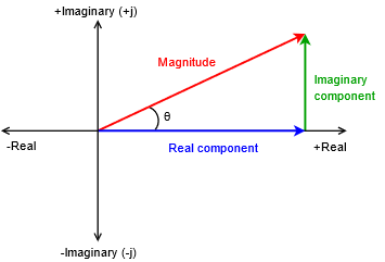
In AC circuits, parameters such as voltage and current are vectors, that is, they have both a magnitude and a phase shift or angle. For example, a voltage might be “12 volts at an angle of 30 degrees” (or more compactly, \(12\angle 30^{\circ}\)). This is known as polar form or magnitude-angle form. Alternately, a vector can be broken into rectangular form, that is, its right angle components.

This can be visualized as a right triangle where the magnitude is the hypotenuse, the angle is the rotation above or below the horizontal, the horizontal component is the side adjacent to the angle and the vertical component is the side opposite of the angle. This is shown in Figure \(\PageIndex{1}\).

Figure \(\PageIndex{1}\): Polar and rectangular forms.

Properly, voltage and current vectors are complex numbers that lay on a complex plane consisting of a real part and an imaginary part. The horizontal axis is the real number axis and the vertical axis is the imaginary number axis. The imaginary axis denotes values times the imaginary operator \(j\) (and often referred to as \(i\) outside of electrical analysis). The \(j\) operator is the square root of −1. An example of such a value is \(3 + j4\), in other words, 3 units along the horizontal real axis and 4 units up the vertical imaginary axis. This is depicted in Figure \(\PageIndex{2}\).

Figure \(\PageIndex{2}\): Polar and rectangular forms on the complex plane.

Converting from one form to another relies on basic trigonometric relations. For convenience, the relationships between the magnitude, angle, real component and imaginary component are reproduced below:

\[\text{Magnitude } = \sqrt{\text{Real}^2 + \text{Imaginary}^2} \label{1.6a} \]

\[\theta = \tan^{−1} \frac{\text{Imaginary}}{\text{Real}} \label{1.6b} \]

\[\text{Real } = \text{ Magnitude } \cos \theta \label{1.6c} \]

\[j\text{Imaginary } = \text{ Magnitude } \sin \theta \label{1.6d} \]

To add or subtract complex quantities, first put them into rectangular form and then combine the reals with the reals and the \(j\) terms with the \(j\) terms as in \((3 + j5) + (13 − j1) = 16 + j4\). These real and imaginary terms must be kept separate. \(3 + j5\) does not equal 8 (or even \(j8\)). That would be like saying that moving 3 feet to your right and 5 feet forward puts you in the same location as moving 8 feet to your right (or 8 feet forward).

The direct way to multiply or divide complex values is to first put them in polar form and then multiply or divide the magnitudes. The angles are added together for multiplication and subtracted for division. For example, \(12\angle 30^{\circ}\) times \(2\angle 45^{\circ}\) is \(24\angle 75^{\circ}\) while dividing them yields \(6\angle −15^{\circ}\). The need for complex numbers will become more obvious as we move through the upcoming material. It is imperative that you have mastered the manipulation of complex values before moving on to subsequent chapters.

You can find out more details from the introduction of phasor video.

Example \(\PageIndex{1}\)

Convert \(15 + j20\) and \(1 k − j2 k\) into polar form, and \(10\angle 45^{\circ}\) and \(0.2\angle −30^{\circ}\) into rectangular form.

For the first two conversions, use Equations \ref{1.6a} and \ref{1.6b}.

\[\text{Magnitude } = \sqrt{15^2 + 20^2} = 25 \nonumber \]

\[\theta = \tan^{−1} \left( \frac{20}{15} \right) = 53.1^{\circ} \nonumber \]

\[\text{Magnitude } = \sqrt{1 k^2 + (−2 k)^2} = 2.236 k \nonumber \]

\[\theta = \tan^{−1} \left( \frac{−2k}{1 k} \right) = −63.4^{\circ} \nonumber \]

The answers for the first part are \(25\angle 53.1^{\circ}\) and \(2.236 k\angle −63.4^{\circ}\).

For the second pair of conversions use Equations \ref{1.6c} and \ref{1.6d}.

\[\text{Real } = 10 \cos 45^{\circ} = 7.07 \nonumber \]

\[j\text{Imaginary } = 10 \sin 45^{\circ} = j 7.07 \nonumber \]

\[\text{Real } = 0.2 \cos −30^{\circ} = 0.173 \nonumber \]

\[j\text{Imaginary } = 0.2 \sin −30^{\circ} = − j0.1 \nonumber \]

The answers for the second part are \(7.07 + j7.07\) and \(0.173 − j0.1\).

Example \(\PageIndex{2}\)

a) Add \(7 + j8 to + j6\), b) Subtract \(5\angle 53.1^{\circ}\) from \(10\angle −45^{\circ}\), c) Divide \(20\angle 90^{\circ}\) by \(4\angle −50^{\circ}\), d) Multiply \(90 + j75\) by \(6 + j10\).

a) Add real to real and imaginary to imaginary: \(7 + j14\).

b) First convert the values into rectangular: \(3 + j4\) and \(7.07 − j7.07\). Now subtract the first pair from the second pair: \(4.07 − j11.07\) (or \(11.8\angle −69.8^{\circ}\)).

c) Divide the magnitudes and subtract the angles: \(5\angle 140^{\circ}\).

d) First convert the values into polar: \(117.15\angle 39.8^{\circ}\) and \(11.66\angle 59^{\circ}\). Now multiply the magnitudes and add the angles: \(1.366 k\angle 98.8^{\circ}\).