1.4: The Link Layer

The link layer is the bottom-most of the three layers of our reference model. The link layer is responsible for moving data directly from one physical location to another. It thus gets involved in several distinct issues: physical transmission, framing bits and bit sequences, detecting transmission errors, multiplexing the link, and providing a useful interface to the network layer above.

Transmitting Digital Data in an Analog World

The purpose of the link layer is to move bits from one place to another. If we are talking about moving a bit from one register to another on the same chip, the mechanism is fairly simple: run a wire that connects the output of the first register to the input of the next. Wait until the first register’s output has settled and the signal has propagated to the input of the second; the next clock tick reads the data into the second register. If all of the voltages are within their specified tolerances, the clock ticks are separated enough in time to allow for the propagation, and there is no electrical interference, then that is all there is to it.

Maintaining those three assumptions is relatively easy within a single chip, and even between chips on the same printed circuit board. However, as we begin to consider sending bits between boards, across the room, or across the country, these assumptions become less and less plausible, and they must be replaced with explicit measures to ensure that data is transmitted accurately. In particular, when the sender and receiver are in separate systems, providing a correctly timed clock signal becomes a challenge.

Figure \(\PageIndex{1}\): A simple protocol for data acknowledge communication.

A simple method for getting data from one module to another module that does not share the same clock is with a three-wire (plus common ground) ready/acknowledge protocol, as shown in Figure \(\PageIndex{1}\). Module \(A\), when it has a bit ready to send, places the bit on the data line, and then changes the steady-state value on the ready line. When \(B\) sees the ready line change, it acquires the value of the bit on the data line, and then changes the acknowledge line to tell \(A\) that the bit has been safely received. The reason that the ready and acknowledge lines are needed is that, in the absence of any other synchronizing scheme, \(B\) needs to know when it is appropriate to look at the data line, and \(A\) needs to know when it is safe to stop holding the bit value on the data line. The signals on the ready and acknowledge lines frame the bit.

If the propagation time from \(A\) to \(B\) is \(\Delta t\), then this protocol would allow \(A\) to send one bit to \(B\) every \(2 \Delta t\) plus the time required for \(A\) to set up its output and for \(B\) to acquire its input, so the maximum data rate would be a little less than \(1/(2 \Delta t)\). Over short distances, one can replace the single data line with \(N\) parallel data lines, all of which are framed by the same pair of ready/acknowledge lines, and thereby increase the data rate to \(N/(2 \Delta t)\). Many backplane bus designs, as well as peripheral attachment systems such as SCSI and personal computer printer interfaces, use this technique, known as parallel transmission, along with some variant of a ready/acknowledge protocol to achieve a higher data rate.

However, as the distance between \(A\) and \(B\) grows, \(\Delta t\) also grows and the maximum data rate declines in proportion, so the ready/acknowledge technique rapidly breaks down. The usual requirement is to send data at higher rates over longer distances with fewer wires, and this requirement leads to employment of a different system called serial transmission. The idea is to send a stream of bits down a single transmission line, without waiting for any response from the receiver and with the expectation that the receiver will somehow recover those bits at the other end with no additional signaling. Thus the output at the transmitting end of the link looks like Figure \(\PageIndex{2}\).

Figure \(\PageIndex{2}\): Outgoing serial transmission.

Unfortunately, because the underlying transmission line is analog, the farther these bits travel down the line, the more attenuation, noise, and line-charging effects they suffer. By the time they arrive at the receiver they will be little more than pulses with exponential leading and trailing edges, as suggested by Figure \(\PageIndex{3}\). The receiving module, \(B\), now has a significant problem in understanding this transmission: because it does not have a copy of the clock that \(A\) used to create the bits, it does not know exactly when to sample the incoming line.

Figure \(\PageIndex{3}\): Bit shape deterioration with distance.

A typical solution involves having the two ends agree on an approximate data rate, so that the receiver can run a voltage-controlled oscillator (VCO) at about that same data rate. The output of the VCO is multiplied by the voltage of the incoming signal and the product suitably filtered and sent back to adjust the VCO. If this circuit is designed correctly, it will lock the VCO to both the frequency and phase of the arriving signal. (This device is commonly known as a phase-locked loop.) The VCO, once locked, then becomes a clock source that a receiver can use to sample the incoming data.

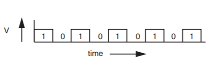
One complication is that with certain patterns of data (for example, a long string of zeros) there may be no transitions in the data stream, in which case the phase-locked loop will not be able to synchronize. To deal with this problem, the transmitter usually encodes the data in a way that ensures that no matter what pattern of bits is sent, there will be some transitions on the transmission line. A frequently used method is called phase encoding, in which there is at least one level transition associated with every data bit. A common phase encoding is the Manchester code, in which the transmitter encodes each bit as two bits: a zero is encoded as a zero followed by a one, while a one is encoded as a one followed by a zero. This encoding guarantees that there is a level transition in the center of every transmitted bit, thus supplying the receiver with plenty of clocking information. It has the disadvantage that the maximum data rate of the communication channel is effectively cut in half, but the resulting simplicity of both the transmitter and the receiver is often worth this price. Other, more elaborate, encoding schemes can ensure that there is at least one transition for every few data bits. These schemes don’t reduce the maximum data rate as much, but they complicate encoding, decoding, and synchronization.

The usual goal for the design space of a physical communication link is to achieve the highest possible data rate for the encoding method being used. That highest possible data rate will occur exactly at the point where the arriving data signal is just on the ragged edge of being correctly decodable, and any noise on the line will show up in the form of clock jitter or signals that just miss expected thresholds, either of which will lead to decoding errors.

Sidebar \(\PageIndex{1}\)

Framing phase-encoded bits

The astute reader may have spotted a puzzling gap in the brief description of the Manchester code: while it is intended as a way of framing bits as they appear on the transmission line, it is also necessary to frame the data bits themselves, in order to know whether a data bit is encoded as the bits \( (n, n+1)\) or the bits \((n+1, n+2)\). A typical approach is to combine code bit framing with data bit framing (and even provide some help in higher-level framing) by specifying that every transmission must begin with a standard pattern, such as some minimum number of coded one-bits followed by a coded zero. The series of consecutive ones gives the Phase-Locked Loop something to synchronize on, and at the same time provides examples of the positions of known data bits. The zero frames the end of the framing sequence. 

The data rate of a digital link is conventionally measured in bits per second. Since digital data is ultimately carried using an analog channel, the question arises of what might be the maximum digital carrying capacity of a specified analog channel. A perfect analog channel would have an infinite capacity for digital data because one could both set and measure a transmitted signal level with infinite precision, and then change that setting infinitely often. In the real world, noise limits the precision with which a receiver can measure the signal value, and physical limitations of the analog channel such as chromatic dispersion (in an optical fiber), charging capacitance (in a copper wire), or spectrum availability (in a wireless signal) put a ceiling on the rate at which a receiver can detect a change in value of a signal. These physical limitations are summed up in a single measure known as the bandwidth of the analog channel. To be more precise, the number of different signal values that a receiver can distinguish is proportional to the logarithm of the ratio of the signal power to the noise power, and the maximum rate at which a receiver can distinguish changes in the signal value is proportional to the analog bandwidth.

These two parameters (signal-to-noise ratio and analog bandwidth) allow one to calculate a theoretical maximum possible channel capacity (that is, data transmission rate) using Shannon's capacity theorem (see Sidebar \(\PageIndex{2}\)).\(^*\) Although this formula adopts a particular definition of bandwidth, assumes a particular randomness for the noise, and says nothing about the delay that might be encountered if one tries to operate near the channel capacity, it turns out to be surprisingly useful for estimating capacities in the real world.

Sidebar \(\PageIndex{2}\)

Shannon's capacity theorem

\[ C \leq W \cdot \log _2 \left( 1 + \frac{S}{NW} \right), \text{ where:} \]

\begin{align*} &C \ = \text{channel capacity, in bits per second} \\    &W = \text{channel bandwidth, in hertz} \\    &S \ = \text{maximum allowable signal power, as seen by the receiver} \\   &N \ = \text{noise power per unit of bandwidth} \end{align*}

Since some methods of digital transmission come much closer to Shannon's theoretical capacity than others, it is customary to use as a measure of goodness of a digital transmission system the number of bits per second that the system can transmit per hertz of bandwidth. Setting \(W = 1\), the capacity theorem says that the maximum bits per second per hertz is \(\log _2 (1 + S/N)\). An elementary signaling system in a low-noise environment can easily achieve 1 bit per second per hertz. On the other hand, for a 28 kilobits per second modem to operate over the 2.4 kilohertz telephone network, it must transmit about 12 bits per second per hertz. The capacity theorem says that the logarithm must be at least 12, so the signal-to-noise ratio must be at least 2¹², or using a more traditional analog measure, 36 decibels, which is just about typical for the signal-to-noise ratio of a properly working telephone connection. The copper-pair link between a telephone handset and the telephone office does not go through any switching equipment, so it actually has a bandwidth closer to 100 kilohertz and a much better signal-to-noise ratio than the telephone system as a whole; these combine to make possible "digital subscriber line" (DSL) modems that operate at 1.5 megabits/second—and even up to 50 megabits/second over short distances—using a physical link that was originally designed to carry just voice.

One other parameter is often mentioned in characterizing a digital transmission system: the bit error rate, abbreviated BER and measured as a ratio to the transmission rate. For a transmission system to be useful, the bit error rate must be quite low; it is typically reported with numbers such as one error in 10⁶, 10⁷, or 10⁸ transmitted bits. Even the best of those rates is not good enough for digital systems; higher levels of the system must be prepared to detect and compensate for errors.

---

\(^*\) The derivation of this theorem is beyond the scope of this textbook. The capacity theorem was originally proposed by Claude E. Shannon in the paper "A mathematical theory of communication," Bell System Technical Journal 27 (1948), pages 379–423 and 623–656. Most modern texts on information theory explore it in depth.

 

Framing Frames

The previous section explained how to obtain a stream of neatly framed bits, but because the job of the link layer is to deliver frames across the link, it must also be able to figure out where in this stream of bits each frame begins and ends. Framing frames is a distinct, and quite independent, requirement from framing bits, and it is one of the reasons that some network models divide the link layer into two layers—a lower layer that manages physical aspects of sending and receiving individual bits and an upper layer that implements the strategy of transporting entire frames.

There are many ways to frame frames. One simple method is to choose some pattern of bits—for example, seven one-bits in a row—as a frame-separator mark. The sender simply inserts this mark into the bit stream at the end of each frame. Whenever this pattern appears in the received data, the receiver takes it to mark the end of the previous frame, and assumes that any bits that follow belong to the next frame. This scheme works nicely, as long as the payload data stream never contains the chosen pattern of bits.

Rather than explaining to the higher layers of the network that they cannot transmit certain bit patterns, the link layer implements a technique known as bit stuffing. The transmitting end of the link layer, in addition to inserting the frame-separator mark between frames, examines the data stream itself, and if it discovers six ones in a row it stuffs an extra bit into the stream, a zero. The receiver, in turn, watches the incoming bit stream for long strings of ones. When it sees six one-bits in a row it examines the next bit to decide what to do. If the seventh bit is a zero, the receiver discards the zero bit, thus reversing the stuffing done by the sender. If the seventh bit is a one, the receiver takes the seven ones as the frame separator. Figure \(\PageIndex{4}\) shows a simple pseudocode implementation of the procedure to send a frame with bit stuffing, and Figure \(\PageIndex{5}\) shows the corresponding procedure on the receiving side of the link. (For simplicity, the illustrated receive procedure ignores two important considerations. First, the receiver uses only one frame buffer. A better implementation would have multiple buffers to allow it to receive the next frame while processing the current one. Second, the same thread that acquires a bit also runs the network level protocol by calling LINK_RECEIVE. A better implementation would probably NOTIFY a separate thread that would then call the higher-level protocol, and this thread could continue processing more incoming bits.)

Figure \(\PageIndex{4}\): Sending a frame with bit stuffing.

Figure \(\PageIndex{5}\): Receiving a frame with bit stuffing.

Bit stuffing is one of many ways to frame frames. There is little need to explore all the possible alternatives because frame framing is easily specified and subcontracted to the implementer of the link layer—the entire link layer, along with bit framing, is often done in the hardware—so we now move on to other issues.

 

Error Handling

An important issue is what the receiving side of the link layer should do about bits that arrive with doubtful values. Since the usual design pushes the data rate of a transmission link up until the receiver can barely tell the ones from the zeros, even a small amount of extra noise can cause errors in the received bit stream.

The first and perhaps most important line of defense in dealing with transmission errors is to require that the design of the link be good at detecting such errors when they occur. The usual method is to encode the data with an error detection code, which entails adding a small amount of redundancy. A simple form of such a code is to have the transmitter calculate a checksum and place the checksum at the end of each frame. As soon as the receiver has acquired a complete frame, it recalculates the checksum and compares its result with the copy that came with the frame. By carefully designing the checksum algorithm and making the number of bits in the checksum large enough, one can make the probability of not detecting an error as low as desired. The more interesting issue is what to do when an error is detected. There are three alternatives:

1. Have the sender encode the transmission using an error correction code, which is a code that has enough redundancy to allow the receiver to identify the particular bits that have errors and correct them. This technique is widely used in situations where the noise behavior of the transmission channel is well understood and the redundancy can be targeted to correct the most likely errors. For example, compact disks are recorded with a burst error-correction code designed to cope particularly well with dust and scratches. Error correction is one of the topics of Chapter 2.
2. Ask the sender to retransmit the frame that contained an error. This alternative requires that the sender hold the frame in a buffer until the receiver has had a chance to recalculate and compare its checksum. The sender needs to know when it is safe to reuse this buffer for another frame. In most such designs the receiver explicitly acknowledges the correct (or incorrect) receipt of every frame. If the propagation time from sender to receiver is long compared with the time required to send a single frame, there may be several frames in flight, and acknowledgments (especially the ones that ask for retransmission) are disruptive. On a high-performance link, an explicit acknowledgment system can be surprisingly complex.
3. Let the receiver discard the frame. This alternative is a reasonable choice in light of our previous observation (see Section 1.2.3) that congestion in higher network levels must be handled by discarding packets anyway. Whatever higher-level protocol is used to deal with those discarded packets will also take care of any frames that are discarded because they contained errors.

Real-world designs often involve blending these techniques, for example by having the sender apply a simple error-correction code that catches and repairs the most common errors and that reliably detects and reports any more complex irreparable errors, and then by having the receiver discard the frames that the error-correction code could not repair.

 

The Link Layer Interface: Link Protocols and Multiplexing

The link layer, in addition to sending bits and frames at one end and receiving them at the other end, also has interfaces to the network layer above, as illustrated in Figure \(1.3.5\) in Section 1.3.2. As described so far, the interface consists of an ordinary procedure call (to LINK_SEND) that the network layer uses to tell the link layer to send a packet, and an upcall (to NETWORK_HANDLE ) from the link layer to the network layer at the other end to alert the network layer that a packet arrived. 

To be practical, this interface between the network layer and the link layer needs to be expanded slightly to incorporate two additional features not previously mentioned: multiple lower-layer protocols, and higher-layer protocol multiplexing. To support these two functions we add two arguments to LINK_SEND , named link_protocol and network_protocol :

LINK_SEND (data_buffer, link_identifier, link_protocol, network_protocol)

Over any given link, it is sometimes appropriate to use different protocols at different times. For example, a wireless link may occasionally encounter a high noise level and need to switch from the usual link protocol to a "robustness" link protocol that employs a more expensive form of error detection with repeated retry, but runs more slowly. At other times it may want to try out a new, experimental link protocol. The third argument to LINK_SEND, namely link_protocol , tells LINK_SEND which link protocol to use for this data, and its addition leads to the protocol layering illustrated in Figure \(\PageIndex{6}\).

Figure \(\PageIndex{6}\): Layer composition with multiple link protocols.

The second feature of the interface to the link layer is more involved: the interface should support protocol multiplexing. Multiplexing allows several different network layer protocols to use the same link. For example, Internet Protocol, Appletalk Protocol, and Address Resolution Protocol (we will talk about some of these protocols later in this chapter) might all be using the same link. Several steps are required. First, the network layer protocol on the sending side needs to specify which protocol handler should be invoked on the receiving side, so one more argument, network_protocol , is needed in the interface to LINK_SEND.

Second, the value of network_protocol needs to be transmitted to the receiving side, for example by adding it to the link-level packet header. Finally, the link layer on the receiving side needs to examine this new header field to decide to which of the various network layer implementations it should deliver the packet. Our protocol layering organization is now as illustrated in Figure \(\PageIndex{7}\). This figure demonstrates the real power of the layered organization: any of the four network layer protocols in the figure may use any of the three link layer protocols.

Figure \(\PageIndex{7}\): Layer composition with multiple link protocols and link layer multiplexing to support multiple network layer protocols.

With the addition of multiple link protocols and link multiplexing, we can summarize the discussion of the link layer in the form of pseudocode for the procedures LINK_SEND and LINK_RECEIVE , together with a structure describing the frame that passes between them, as in Figure \(\PageIndex{8}\). In procedure LINK_SEND, the procedure variable sendproc is selected from an array of link layer protocols; the value found in that array might be, for example, a version of the procedure PACKET_TO_BIT of Figure \(\PageIndex{5}\) that has been extended with a third argument that identifies which link to use. The procedures CHECKSUM and LENGTH are programs we assume are found in the library. Procedure LINK_RECEIVE might be called, for example, by procedure BIT_TO_FRAME of Figure \(\PageIndex{5}\). The procedure LINK_RECEIVE verifies the checksum, and then

extracts net_data and net_protocol from the frame and passes them to the procedure that calls the network handler together with the identifier of the link over which the packet arrived.

Figure \(\PageIndex{8}\): The LINK_SEND and LINK_RECEIVE procedures, together with the structure of the frame transmitted over the link and a dispatching procedure for the network layer.

These procedures also illustrate an important property of layering that was discussed in Section 1.3.4. The link layer handles its argument data_buffer as an unstructured string of bits. When we examine the network layer in the next section of the chapter, we will see that data_buffer contains a network-layer packet, which has its own internal structure. The point is that as we pass from an upper layer to a lower layer, the content and structure of the payload data is not supposed to be any concern of the lower layer.

As an aside, the division we have chosen for our sample implementation of a link layer, with one program doing framing and another program verifying checksums, corresponds to the OSI reference model division of the link layer into physical and strategy layers, as was mentioned in Section 1.3.5.

Since the link is now multiplexed among several network-layer protocols, when a frame arrives, the link layer must dispatch the packet contained in that frame to the proper network layer protocol handler. Figure \(\PageIndex{8}\) shows a

handler dispatcher named GIVE_TO_NETWORK_HANDLER. Each of several different network-layer protocol-implementing programs specifies the protocol it knows how to handle, through arguments in a call to SET_HANDLER. Control then passes to a particular network-layer handler only on arrival of a frame containing a packet of the protocol it specified. With some additional effort (not illustrated—the reader can explore this idea as an exercise), one could also make this dispatcher multithreaded, so that as it passes a packet up to the network layer a new thread takes over and the link layer thread returns to work on the next arriving frame.

With or without threads, the network_protocol field of a frame indicates to whom in the network layer the packet contained in the frame should be delivered. From a more general point of view, we are multiplexing the lower-layer protocol among several higher-layer protocols. This notion of multiplexing, together with an identification field to support it, generally appears in every protocol layer, and in every layer-to-layer interface, of a network architecture.

An interesting challenge is that the multiplexing field of a layer names the protocols of the next higher layer, so some method is needed to assign those names. Since higher-layer protocols are likely to be defined and implemented by different organizations, the usual solution is to hand the name conflict avoidance problem to some national or international standard-setting body. For example, the names of the protocols of the Internet are assigned by an outfit called ICANN, which stands for the Internet Corporation for Assigned Names and Numbers.

 

Link Properties

Some final details complete our tour of the link layer. First, links come in several flavors, for which there is some standard terminology:

A point-to-point link directly connects exactly two communicating entities. A simplex link has a transmitter at one end and a receiver at the other; two-way communication requires installing two such links, one going in each direction. A duplex link has both a transmitter and a receiver at each end, allowing the same link to be used in both directions. A half-duplex link is a duplex link in which transmission can take place in only one direction at a time, whereas a full-duplex link allows transmission in both directions at the same time over the same physical medium.

A broadcast link is a shared transmission medium in which there can be several transmitters and several receivers. Anything sent by any transmitter can be received by many—perhaps all—receivers. Depending on the physical design details, a broadcast link may limit use to one transmitter at a time, or it may allow several distinct transmissions to be in progress at the same time over the same physical medium. This design choice is analogous to the distinction between half duplex and full duplex but there is no standard terminology for it. The link layers of the standard Ethernet and the popular wireless system known as Wi-Fi are one-transmitter-at-a-time broadcast links. The link layer of a CDMA Personal Communication System (such as ANSI–J–STD–008, which is used by cellular providers Verizon and Sprint PCS) is a broadcast link that permits many transmitters to operate simultaneously.

Finally, most link layers impose a maximum frame size, known as the maximum transmission unit (MTU). The reasons for limiting the size of a frame are several:

1. The MTU puts an upper bound on link commitment time, which is the length of time that a link will be tied up once it begins to transmit the frame. This consideration is more important for slow links than for fast ones.
2. For a given bit error rate, the longer a frame is, the greater the chance of an uncorrectable error in that frame. Since the frame is usually also the unit of error control, an uncorrectable error generally means loss of the entire frame, so as the frame length increases not only does the probability of loss increase, but the cost of the loss increases because the entire frame will probably have to be retransmitted. The MTU puts a ceiling on both of these costs.
3. If congestion leads a forwarder to discard a packet, the MTU limits the amount of transmission capacity required to retransmit the packet.
4. There may be mechanical limits on the maximum length of a frame. A hardware interface may have a small buffer or a short counter register tracking the number of bits in the frame. Similar limits sometimes are imposed by software that was originally designed for another application or to comply with some interoperability standard.

Whatever the reason for the MTU, when an application needs to send a message that does not fit in a maximum-sized frame, it becomes the job of some end-to-end protocol to divide the message into segments for transmission and to reassemble the segments into the complete message at the other end. The way in which the end-to-end protocol discovers the value of the MTU is complicated—it needs to know not just the MTU of the link it is about to use, but the smallest MTU that the segment will encounter on the path through the network to its destination. For this purpose, it needs some help from the network layer, which is our next topic.