1.2: Interesting Properties of Networks

The design of communication networks is dominated by three intertwined considerations: (1) a trio of fundamental physical properties, (2) the mechanics of sharing, and (3) a remarkably wide range of parameter values. The first dominating consideration is the trio of fundamental physical properties:

1. The speed of light is finite. Using the most direct route, and accounting for the velocity of propagation in real-world communication media, it takes about 20 milliseconds to transmit a signal across the 2,600 miles from Boston to Los Angeles. This time is known as the propagation delay, and there is no way to avoid it without moving the two cities closer together. If the signal travels via a geostationary satellite perched 22,400 miles above the equator and at a longitude halfway between those two cities, the propagation delay jumps to 244 milliseconds, a latency large enough that a human, not just a computer, will notice. However, communication between two computers in the same room may have a propagation delay of only 10 nanoseconds. That shorter latency makes some things easier to do, but the important implication is that network systems may have to accommodate a range of delay that spans seven orders of magnitude.
2. Communication environments are hostile. Computers are usually constructed of incredibly reliable components, and they are usually operated in relatively benign environments. But communication is carried out using wires, glass fibers, or radio signals that must traverse far more hostile environments ranging from under the floor to deep in the ocean. These environments endanger communication. Threats range from a burst of noise that wipes out individual bits to careless backhoe operators who sever cables that can require days to repair.
3. Communication media have limited bandwidth. Every transmission medium has a maximum rate at which one can transmit distinct signals. This maximum rate is determined by its physical properties, such as the distance between transmitter and receiver and the attenuation characteristics of the medium. Signals can be multilevel, not just binary, so the data rate can be greater than the signaling rate. However, noise limits the ability of a receiver to distinguish one signal level from another. The combination of limited signaling rate, finite signal power, and the existence of noise limits the rate at which data can be sent over a communication link.\(^*\) Different network links may thus have radically different data rates, ranging from a few kilobits per second over a long-distance telephone line to several tens of gigabits per second over an optical fiber. Available data rate thus represents a second network parameter that may range over seven orders of magnitude.

\(^*\) The formula that relates signaling rate, signal power, noise level, and maximum data rate, known as Shannon’s capacity theorem, appears in Sidebar 2 in Section 1.4. 

---

The second dominating consideration of communications networks is that they are nearly always shared. Sharing arises for two distinct reasons.

1. Any-to-any connection. Any communication system that connects more than two things intrinsically involves an element of sharing. If you have three computers, you usually discover quickly that there are times when you want to communicate between any pair. You can start by building a separate communication path between each pair, but this approach runs out of steam quickly because the number of paths required grows with the square of the number of communicating entities. Even in a small network, a shared communication system is usually much more practical—it is more economical and it is easier to manage. When the number of entities that need to communicate begins to grow, as suggested in Figure \(\PageIndex{1}\), there is little choice. A closely related observation is that networks may connect three entities or 300 million entities. The number of connected entities is thus a third network parameter with a wide range, in this case covering eight orders of magnitude.
2. Sharing of communication costs. Some parts of a communication system follow the same technological trends as do processors, memory, and disk: things made of silicon chips seem to fall in price every year. Other parts, such as digging up streets to lay wire or fiber, launching a satellite, or bidding to displace an existing radiobased service, are not getting any cheaper. Worse, when communication links leave a building, they require right-of-way, which usually subjects them to some form of regulation. Regulation operates on a majestic time scale, with procedures that involve courts and attorneys, legislative action, long-term policies, political pressures, and expediency. These procedures can eventually produce useful results, but on time scales measured in decades, whereas technological change makes new things feasible every year. This incommensurate rate of change means that communication costs rarely fall as fast as technology would permit, so sharing of those costs between otherwise independent users persists even in situations where the technology might allow them to avoid it.

The third dominating consideration of network design is the wide range of parameter values. We have already seen that propagation times, data rates, and the number of communicating computers can each vary by seven or more orders of magnitude. There is a fourth such wide-ranging parameter: a single computer may at different times present a network with widely differing loads, ranging from transmitting a file at 30 megabytes per second to interactive typing at a rate of one byte per second.

These three considerations, unyielding physical limits, sharing of facilities, and existence of four different parameters that can each range over seven or more orders of magnitude, intrude on every level of network design, and even carefully thought-out modularity cannot completely mask them. As a result, systems that use networks as a component must take them into account. 

Isochronous and Asynchronous Multiplexing

Sharing has significant consequences. Consider the simplified (and gradually becoming obsolescent) telephone network of Figure \(\PageIndex{1}\), which allows telephones in Boston to talk with telephones in Los Angeles. There are three shared components in this picture: a switch in Boston, a switch in Los Angeles, and an electrical circuit acting as a communication link between the two switches. The communication link is multiplexed, which means simply that it is used for several different communications at the same time. Let's focus on the multiplexed link. Suppose that there is an earthquake in Los Angeles, and many people in Boston simultaneously try to call their relatives in Los Angeles to find out what happened. The multiplexed link has a limited capacity, and at some point the next caller will be told the "network is busy." (In the U.S. telephone network this event is usually signaled with "fast busy," a series of beeps repeated at twice the speed of a usual busy signal.)

Figure \(\PageIndex{1}\): A simple telephone network.

This "network busy" phenomenon strikes rather abruptly because the telephone system traditionally uses a line multiplexing technique known as isochronous (from Greek roots meaning "equally timed") communication. Suppose that the telephones are all digital, operating at 64 kilobits per second, and the multiplexed link runs at 45 megabits per second. If we look for the bits that represent the conversation between \(B_2\) and \(L_3\), we will find them on the wire as shown in Figure \(\PageIndex{2}\): At regular intervals we will find 8-bit blocks (called frames) carrying data from \(B_2\) to \(L_3\). To maintain the required data rate of 64 kilobits per second, another \(B_2\)-to-\(L_3\) frame comes by every 5,624 bit times or 125 microseconds, producing a rate of 8,000 frames per second. In between each pair of \(B_2\)-to-\(L_3\) frames there is room for 702 other frames, which may be carrying bits belonging to other telephone conversations. A 45 megabits/second link can thus carry up to 703 simultaneous conversations, but if a 704^th person tries to initiate a call, that person will receive the “network busy” signal. Such a capacity-limiting scheme is sometimes called hard-edged, meaning in this case that it offers no resistance to the first 703 calls, but it absolutely refuses to accept the 704^th one.

Figure \(\PageIndex{2}\): Data flow on an isochronous multiplexed link.

This scheme of dividing up the data into equal-size frames and transmitting the frames at equal intervals—known in communications literature as time-division multiplexing (TDM)—is especially suited to telephony because, from the point of view of any one telephone conversation, it provides a constant rate of data flow and the delay from one end to the other is the same for every frame.

One prerequisite to using isochronous communication is that there must be some prior arrangement between the sending switch and the receiving switch: an agreement that this periodic series of frames should be sent along to \(L_3\). This agreement is an example of a connection and it requires some previous communication between the two switches to set up the connection, storage for remembered state at both ends of the link, and some method to discard (tear down) that remembered state when the conversation between \(B_2\) and \(L_3\) is complete.

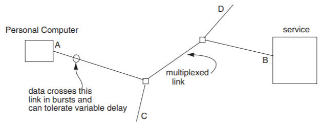
Data communication networks usually use a strategy different from telephony for multiplexing shared links. The starting point for this different strategy is to examine the data rate and latency requirements when one computer sends data to another. Usually, computer-related activities send data on an irregular basis—in bursts called messages—as compared with the continuous stream of bits that flows out of a simple digital telephone. Bursty traffic is particularly ill-suited to fixed size and spacing of isochronous frames. During those times when \(B_2\) has nothing to send to \(L_3\), the frames allocated to that connection go unused. Yet when \(B_2\) does have something to send it may be larger than one frame in size, in which case the message may take a long time to send because of the rigidly fixed spacing between frames. Even if intervening frames belonging to other connections are unfilled, they can’t be used by the connection from \(B_2\) to \(L_3\). When communicating data between two computers, a system designer is usually willing to forgo the guarantee of uniform data rate and uniform latency if in return an entire message can get through more quickly. Data communication networks achieve this trade-off by using what is called asynchronous (from Greek roots meaning “untimed”) multiplexing. For example, in Figure \(\PageIndex{3}\), a network connects several personal computers and a service. In the middle of the network is a 45 megabits/second multiplexed link, shared by many network users. But, unlike the telephone example, this link is multiplexed asynchronously.

Figure \(\PageIndex{3}\): A simple data communication network.

On an asynchronous link, a frame can be of any convenient length, and can be carried at any time that the link is not being used for another frame. Thus in the time sequence shown in Figure \(\PageIndex{4}\) we see two frames, the first going to \(B\) and the second going to \(D\). Since the receiver can no longer figure out where the message in the frame is destined by simply counting bits, each frame must include a few extra bits that provide guidance about where to deliver it. A variable-length frame, together with its guidance information, is called a packet. The guidance information can take any of several forms. A common form is to provide the destination address of the message: the name of the place to which the message should be delivered. In addition to delivery guidance information, asynchronous data transmission requires some way of figuring out where each frame starts and ends, a process known as framing. In contrast, both addressing and framing with isochronous communication are done implicitly, by watching the clock.

Figure \(\PageIndex{4}\): Data flow on an asynchronous multiplexed link.

Since a packet carries its own destination guidance, there is no need for any prior agreement between the ends of the multiplexed link. Asynchronous communication thus offers the possibility of connectionless transmission, in which the switches do not need to maintain state about particular end-user communications.\(^*\)

An additional complication arises because most links place a limit on the maximum size of a frame. When a message is larger than this maximum size, it is necessary for the sender to break it up into segments, each of which the network carries in a separate packet, and include enough information with each segment to allow the original message to be reassembled at the other end.

Asynchronous transmission can also be used for continuous streams of data, such as that from a digital telephone, by breaking the stream up into segments. Doing so does create a problem: the segments may not arrive at the other end at a uniform rate or with a uniform delay. On the other hand, if the variations in rate and delay are small enough, or the application can tolerate occasional missing segments of data, the method is still effective. In the case of telephony, the technique is called "packet voice" and it is gradually replacing many parts of the traditional isochronous voice network.

---

\(^*\) Network experts make a subtle distinction among different kinds of packets by using the word datagram to describe a packet that carries all of the state information (for example, its destination address) needed to guide the packet through a network of packet forwarders that do not themselves maintain any state about particular end-to-end connections.

 

Packet Forwarding; Delay

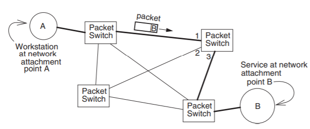
Asynchronous communication links are usually organized in a communication structure known as a packet forwarding network. In this organization, a number of slightly specialized computers known as packet switches (in contrast with the circuit switches of Figure \(\PageIndex{1}\)) are placed at convenient locations and interconnected with asynchronous links. Asynchronous links may also connect customers of the network to network attachment points, as in Figure \(\PageIndex{5}\). This figure shows two attachment points, named \(A\) and \(B\), and it is evident that a packet going from \(A\) to \(B\) may follow any of several different paths, called routes, through the network. Choosing a particular path for a packet is known as routing. The upper right packet switch has three numbered links connecting it to three other packet switches. The packet coming in on its link #1, which originated at the workstation at attachment point \(A\) and is destined for the service at attachment point \(B\), contains the address of its destination. By studying this address, the packet switch will be able to figure out that it should send the packet on its way via its link #3. Choosing an outgoing link is known as forwarding, and is usually done by table lookup. The construction of the forwarding tables is one of several methods of routing, so packet switches are also called forwarders or routers. The resulting organization resembles that of the postal service.

Figure \(\PageIndex{5}\): A packet forwarding network.

A forwarding network imposes a delay (known as its transit time) in sending something from \(A\) to \(B\). There are four contributions to transit time, several of which may be different from one packet to the next.

1. Propagation delay. The time required for the signal to travel across a link is determined by the speed of light in the transmission medium connecting the packet switches and the physical distance the signals travel. Although it does vary slightly with temperature, from the point of view of a network designer propagation delay for any given link can be considered constant. (Propagation delay also applies to the isochronous network.)
2. Transmission delay. Since the frame that carries the packet may be long or short, the time required to send the frame at one switch—and receive it at the next switch—depends on the data rate of the link and the length of the frame. This time is known as transmission delay. Although some packet switches are clever enough to begin sending a packet out before completely receiving it (a trick known as cut-through), error recovery is simpler if the switch does not forward a packet until the entire packet is present and has passed some validity checks. Each time the packet is transmitted over another link, there is another transmission delay. A packet going from \(A\) to \(B\) via the dark links in Figure \(\PageIndex{5}\) will thus be subject to four transmission delays: one when \(A\) sends it to the first packet switch, one at each forwarding step, and finally one to transmit it to \(B\).
3. Processing delay. Each packet switch will have to examine the guidance information in the packet to decide to which outgoing link to send it. The time required to figure this out, together with any other work performed on the packet, such as calculating a checksum (see Sidebar \(\PageIndex{1}\)) to allow error detection or copying it to an output buffer that is somewhere else in memory, is known as processing delay. This delay typically has one part that is relatively constant from one packet to the next and a second part that is proportional to the length of the packet. 

   Sidebar \(\PageIndex{1}\)

   Error detection, checksums, and witnesses

   A checksum on a block of data is a stylized kind of error-detection code in which redundant error-detecting information, rather than being encoded into the data itself (as Chapter 2 will explain), is placed in a separate field. A typical simple checksum algorithm breaks the data block up into \(k\)-bit chunks and performs an exclusive OR on the chunks to produce a \(k\)-bit result. (When \(k = 1\), this procedure is called a parity check.) That simple \(k\)-bit checksum would catch any one-bit error, but it would miss some two-bit errors, and it would not detect that two chunks of the block have been interchanged. Much more sophisticated checksum algorithms have been devised that can detect multiple-bit errors or that are good at detecting particular kinds of expected errors. As will be seen in Chapter 5, by using cryptographic techniques it is possible to construct a high-quality checksum with the property that it can detect all changes—even changes that have been intentionally introduced by a malefactor—with near-certainty. Such a checksum is called a witness or fingerprint and is useful for ensuring long-term integrity of stored data. The trade-off is that more elaborate checksums usually require more time to calculate and thus add to processing delay. For that reason, communication systems typically use the simplest checksum algorithm that has a reasonable chance of detecting the expected errors.

4. Queuing delay. When the packet from \(A\) to \(B\) arrives at the upper right packet switch, link #3 may already be transmitting another packet, perhaps one that arrived from link #2, and there may also be other packets queued up waiting to use link #3. If so, the packet switch will hold the arriving packet in a queue in memory until it has finished transmitting the earlier packets. The duration of this delay depends on the amount of other traffic passing through that packet switch, so it can be quite variable.

Queuing delay can sometimes be estimated with queuing theory (not discussed in this text). If packets arrive according to a random, memoryless process and have randomly distributed service times (technically, a Poisson distribution in which for this case the service time is the transmission delay of the outgoing link), the average queuing delay, measured in units of the packet service time and including the service time of this packet, will be \(1 ⁄ (1 - \rho)\). Here \(\rho\) is the utilization of the outgoing line, which can range from 0 to 1. When we plot this result in Figure \(\PageIndex{6}\) we notice a typical system phenomenon: delay rises rapidly as the line utilization approaches 100%. This plot tells us that the asynchronous system has introduced a trade-off: if we wish to limit the average queuing delay, for example to the amount labeled in the figure "maximum tolerable delay," it will be necessary to leave unused, on average, some of the capacity of each link; in the example this maximum utilization is labeled \(\rho_{max}\). Alternatively, if we allow the utilization to approach 100%, delays will grow without bound. The asynchronous system seems to have replaced the abrupt appearance of the busy signal of the isochronous network with a gradual trade-off: as the system becomes busier, the delays increase. However, as we will see in Section \(\PageIndex{3}\) below, the replacement is actually more subtle than that.

Figure \(\PageIndex{6}\): Queuing delay as a function of utilization.

The formula and accompanying graph tell us only the average delay. If we try to load up a link so that its utilization is \(\rho_{max}\), the actual delay will exceed our tolerance threshold about as often as it is below that threshold. If we are serious about keeping the maximum delay almost always below a given value, we must prepare for occasional worse peaks by holding utilization below the level of \(\rho_{max}\) suggested by the figure. If packets do not obey memoryless arrival statistics (for example, they arrive in long convoys, and all are the same, maximum size), the model no longer applies, and we need a better understanding of the arrival process before we can say anything about delays. This same utilization versus delay trade-off also applies to non-network components of a computer system that have queues: for example, scheduling the processor or reading and writing a magnetic disk.

We have talked about queuing theory as if it might be useful in predicting the behavior of a network. It is not. In practice, network systems put a bound on link queuing delays by limiting the size of queues and by exerting control on arrivals. These mechanisms allow individual links to achieve high utilization levels, while shifting delays to other places in the network. The next section explains how, and it also explains just what happened to the isochronous network’s hard-edged busy signal. Later, in Section 1.7 of this chapter, we will see how the delays can be shifted all the way back to the entry point of the network.

 

Buffer Overflow and Discarded Packets

Continuing for a moment to apply queuing theory, queuing has an implication: buffer space is needed to hold the queue of packets waiting for transmission. How large a buffer should the designer allocate? Under the memoryless arrival interval assumption, the average number of packets awaiting transmission (including the one currently being transmitted) is \(1 / (1-\rho) \). As with queuing delay, that number is only the average—queuing theory tells us that the variance of the queue length is also \(1 / (1-\rho) \). For a \(\rho\) of 0.8 the average queue length and the variance are both 5, so if one wishes to allow enough buffers to handle peaks that are, say, three standard deviations above the average, one must be prepared to buffer not only the 5 packets predicted as the average but also \((3 \times \sqrt{5} \simeq 7)\) more, a total of 12 packets. Worse, in many real networks packets don’t actually arrive independently at random; they come in buffer-bursting batches.

At this point, we can imagine three quite different strategies for choosing a buffer size:

1. Plan for the worst case. Examine the network traffic carefully, figure out what the worst-case traffic situation will be, and allocate enough buffers to handle it.
2. Plan for the usual case and fight back. Based on a calculation such as the one above, choose a buffer size that will work most of the time, and if the buffers fill up send messages back through the network asking someone to stop sending.
3. Plan for the usual case and discard overflow. Again, choose a buffer size that will work most of the time, and ruthlessly discard packets when the buffers are full.

Let’s explore these three possibilities in turn.

Buffer memory is usually low in cost, so planning for the worst case seems like an attractive idea, but it is actually much harder than it sounds. For one thing, in a large network, it may be impossible to figure out what the worst case is—there just isn’t enough information available about what can happen. Even if one can estimate the worst case, the estimate may not be useful. Consider, for example, the Hypothetical Bank of Canada, which has 21,000 tellers scattered across the country. The branch at Moose Jaw, Saskatchewan, has one teller and usually is the target of only three transactions a day. Although it has never happened, and almost certainly never will, the worst case is that every one of the 20,999 other tellers simultaneously posts a withdrawal against a Moose Jaw account. Thus, a worst-case design would require that there be enough buffers in the packet switch leading to Moose Jaw to handle 20,999 simultaneous messages. The problem with worst-case analysis is that the worst case can be many orders of magnitude larger than the average case, as well as extremely unlikely. Moreover, even if one decided to buy that large a buffer, the resulting queue to process all the transactions would be so long that many of the other tellers would give up in disgust and abort their transactions, so the large buffer wouldn’t really help. 

This observation makes it sound attractive to choose a buffer size based on typical, rather than worst-case, loads. But then there is always going to be a chance that traffic will exceed the average for long enough to run out of buffer space. This situation is called congestion. What to do then?

One idea is to push back. If buffer space begins to run low, send a message back along an incoming link saying "please don't send any more until you hear from me." This message (called a quench request) may go to the packet switch at the other end of that link, or it may go all the way back to the original source that introduced the data into the network. Either way, pushing back is also harder than it sounds. If a packet switch is experiencing congestion, there is a good chance that the adjacent switch is also congested (if it is not already congested, it soon will be if it is told to stop sending data over the link to this switch), and sending an extra message is adding to the congestion. Worse, a set of packet switches configured in a cycle like that of Figure \(\PageIndex{5}\) can easily end up in a form of deadlock (called gridlock when it happens to automobile traffic), with all buffers filled and each switch waiting for the next switch to say that it is OK to start sending again.

One way to avoid deadlock among the packet switches is to send the quench request all the way back to the source. This method is hard too, for at least three reasons. First, it may not be clear which source should be the destination of the quench. In our Moose Jaw example, there are 21,000 different sources, no one of which is, by itself, the cause of (nor capable of doing much about) the problem. Second, such a request may not have any effect because the source you choose to quench is no longer sending anyway. Again in our example, by the time the packet switch on the way to Moose Jaw detects the overload, all of the 21,000 tellers may have already sent their transaction requests, so asking them not to send anything else would accomplish nothing. Third, assuming that the quench message is itself forwarded back through the packet-switched network, it may run into congestion and be subject to queuing delays. The busier the network, the longer it will take to exert control. We are proposing to create a feedback system with delay and should expect to see oscillations. Even if all the data is coming from one source, by the time the quench gets back and the source acts on it, the packets already in the pipeline may exceed the buffer capacity. Controlling congestion by quenching either the adjacent switch or the source is used in various special situations, but as a general technique it is currently an unsolved problem.

The remaining possibility is what most packet networks actually do in the face of congestion: when the buffers fill up, they start throwing packets away. This seems like a somewhat startling thing for a communication system to do because it will disrupt the communication, and eventually each discarded packet will have to be sent again, so the effort to send the packet this far will have been wasted. Nevertheless, this is an action that every packet switching network that is not configured for the worst case must be prepared to take.

Overflowing buffers and discarded packets lead to two remarkable consequences. First, the sender of a packet can interpret the lack of its acknowledgment as a sign that the network is congested, and can in turn reduce the rate at which it introduces new packets into the network. This idea, called automatic rate adaptation, is explored in depth in Section 1.7 of this chapter. The combination of discarded packets and automatic rate adaptation in turn produce the second consequence: simple theoretical models of network behavior based on standard queuing theory do not apply when a service may serve some requests and may discard others. Modeling of networks that have rate adaptation requires a much deeper understanding of the specific algorithms used not just by the network but also by network applications.

In the final analysis, the asynchronous network replaces the hard-edged blocking of the isochronous network with a variable transmission rate that depends on the instantaneous network load. Which scheme for dealing with overload (asynchronous or isochronous) is preferable depends on the application. For some applications it may be better to be told at the outset of a communications attempt to come back later, rather than to be allowed to start work only to encounter such variations in available capacity that it is hard to do anything useful. In other applications it may be more helpful to have some work done, slowly or at variable rates, rather than none at all.

The possibility that a network may actually discard packets to cope with congestion leads to a useful distinction between two kinds of forwarding networks. So far, we have been discussing what is usually described as a best-effort network, which, if it cannot dispatch a packet soon after receipt, may discard it. The alternative design is the guaranteed-delivery network (sometimes called a store-and-forward network, although that term is often applied to all forwarding networks), which takes heroic measures to avoid ever discarding payload data. Guaranteed-delivery networks usually are designed to work with complete messages rather than packets. Typically, a guaranteed-delivery network uses non-volatile storage such as a magnetic disk for buffering, so that it can handle large peaks of message load and can be confident that messages will not be lost even if there is a power failure or the forwarding computer crashes. Also, a guaranteed-delivery network usually, when faced with the prospect of being completely unable to deliver a message (perhaps because the intended recipient has vanished), explicitly returns the message to its originator along with an explanation of why delivery failed. Finally, in keeping with the spirit of not losing a message, a guaranteed-delivery switch usually tracks individual messages carefully to make sure that none are lost or damaged during transmission, for example by a burst of noise. A switch of a best-effort network can be quite a bit simpler than a switch of a guaranteed-delivery network. Since the best-effort network may casually discard packets anyway, it does not need to make any special provisions for retransmitting damaged packets, for preserving packets in transit when the switch crashes and restarts, or for worrying about the case when the link to a destination node suddenly stops accepting data.

The best-effort network is said to provide a best-effort contract to its customers (this contract is defined more carefully in Section \(\PageIndex{7}\) below), rather than a guarantee of delivery. Of course, in the real world there are no absolute guarantees—the real distinction between the two designs is that there is intended to be a significant difference in the probability of undetected loss. When we examine network layering in Section 1.3 of this chapter, it will become apparent that these differences can be characterized another way: guaranteed-delivery networks are usually implemented in a higher network layer and best-effort networks in a lower network layer.

In these terms, the U.S. Postal Service operates a guaranteed delivery system for first-class mail, but a best-effort system for third-class (junk) mail, because postal regulations allow it to discard third-class mail that is misaddressed or when congestion gets out of hand. The Internet is organized as a best-effort system, but the Internet mechanisms for handling email are designed as a guaranteed delivery system. The Western Union company has always prided itself on operating a true guaranteed-delivery system, to the extent that when it decommissions an office it normally disassembles the site completely in a search for misplaced telegrams. There is a (possibly apocryphal) tale that such a disassembly once discovered a 75-year-old telegram that had fallen behind a water pipe. The company promptly delivered it to the astonished heirs of the original addressee.

 

Duplicate Packets and Duplicate Suppression

As it turns out, discarded packets are not as much of a problem to the higher-level application as one might expect because when a client sends a request to a service, it is always possible that the service is not available, or the service crashed just after receiving the request. So unanswered requests are actually a routine occurrence, and many network protocols include some kind of timer expiration and resend mechanism to recover from such failures. The timing diagram of Figure \(\PageIndex{7}\) illustrates the situation, showing a first packet carrying a request, followed by a packet going the other way carrying the response to the first request. \(A\) has set a timer, indicated by a vertical line, but the arrival of response 1 before the expiration of the timer causes \(A\) to switch off the timer, indicated by the small x. The packet carrying the second request is lost in transit (as indicated by the large X), perhaps having been damaged or discarded by an overloaded forwarder; the timer expires; and \(A\) resends request 2 in the packet labeled request 2'.

Figure \(\PageIndex{7}\): Lost packet recovery.

When a congested forwarder discards a packet, there are two important consequences. First, the client doesn't receive a response as quickly as originally hoped because a timer expiration period has been added to the overall response time. This extra delay can have a significant impact on performance. Second, users of the network must be prepared for duplicate requests and responses. The reason lies in the recovery mechanism just described. Suppose a network packet switch gets overloaded and must discard a response packet, as in Figure \(\PageIndex{8}\). Client \(A\) can't tell the difference between this case and the case of Figure \(\PageIndex{7}\), so it resends its request. The service sees this resent request as a duplicate. Suppose \(B\) does not realize this is a duplicate, does what is requested, and sends back a response. Client \(A\) receives the response and assumes that everything is OK. That may be a correct assumption, or it may not, depending on whether or not the first arrival of request 3 changed \(B\)'s state. If \(B\) is a spelling checker, it will probably give the same response to both copies of the request. But if \(B\) is a bank and the request is to transfer funds, doing the request twice would be a mistake. So detecting duplicates may or may not be important, depending on the particular application.

Figure \(\PageIndex{8}\): Lost packet recovery leading to duplicate request.

For another example, if for some reason the network delays pile up and exceed the resend timer expiration period, the client may resend a request even though the original response is still in transit. Since \(B\) can’t tell any difference between this case and the previous one, it responds in the same way, by doing what is requested. But now \(A\) receives a duplicate response, as in Figure \(\PageIndex{9}\). Again, this duplicate may or may not matter to \(A\), but at a minimum \(A\) must take steps not to be confused by the arrival of a duplicate response.

Figure \(\PageIndex{9}\): Network delay combined with recovery leading to duplicate response.

What if the arrival of a request from \(A\) causes \(B\) to change state, as in the bank transfer example? If so, it is usually important to detect and suppress duplicates generated by the lost packet recovery mechanism. The general procedure to suppress duplicates has two components. The first component is hinted at by the request and response numbers used in the illustrations: each request includes a nonce, which is a unique identifier that will never be reused by \(A\) when sending requests to \(B\). The illustration uses monotonically increasing serial numbers as nonces, but any unique identifier will do. The second duplicate suppression component is that \(B\) must maintain a list of nonces on which it has taken action or is still working, and whenever a request arrives \(B\) should look through this list to see whether or not this apparently new request is actually a duplicate of one previously received. If it is a duplicate, \(B\) must not perform the action requested. On the other hand, \(B\) should not simply ignore the request, either, because the reason for the duplicate may be that \(A\) never received \(B\)'s response. So, \(B\) needs some way of reconstructing and resending that previous response. The simplest way of doing this is usually for \(B\) to add to its list of previously handled nonces a copy of the corresponding responses so that it can easily resend them. Thus in Figure \(\PageIndex{9}\), the last action of \(B\) should be replaced with "B resends response 4".

In some network designs, \(A\) may even receive duplicate responses to a single, unrepeated request. The reason is that a forwarding link deep inside the network may be using a timer expiration and resend protocol similar to the one above. For this reason, most protocols that are concerned about duplicate suppression include a copy of the nonce in the response, and the originator, \(A\), maintains a list of nonces used in its outstanding requests. When a response comes back, \(A\) can check for the nonce in the list and delete that list entry or, if there is no list entry, assume it is a duplicate of a previously received response and ignore it.

The procedure we have just described allows \(A\) to keep its list of nonces short, but \(B\) might have to maintain an ever-growing list of nonces and responses to be certain that it never accidentally processes a request twice. A related problem concerns what happens if either participant crashes and restarts, losing its volatile memory, which is probably where it is keeping its list of nonces. Refinements to cope with these problems will be explored in detail when we revisit the topic of duplicate suppression in Section 1.6.3 of this chapter.

Ensuring suppression of duplicates is a significant complication. Therefore, if possible it is wise to design the service and its protocol in such a way that suppression is not required. Recall that the reason that duplicate suppression became important was that a request changed the state of the service. It is often possible to design a service interface so that it is idempotent, which for a network request means that repeating the same request or sequence of requests several times has the same effect as doing it just once. This design approach is explored in depth in the discussion of atomicity and error recovery in Chapter 3.

 

Damaged Packets and Broken Links

At the beginning of the chapter we noted that noise is one of the fundamental considerations that dominates the design of data communication. Data can be damaged during transmission, during transit through a switch, or in the memory of a forwarding node. Noise, transmission errors, and techniques for detecting and correcting errors are fascinating topics in their own right, explored in some depth in Chapter 2. As a general rule it is possible to sub-contract this area to a specialist in the theory of error detection and correction, with one requirement in the contract: when we receive data, we want to know whether or not it is correct. That is, we require that a reliable error detection mechanism be part of any underlying data transmission system. Section 1.4 of this chapter expands a bit on this error detection requirement.

Once we have contracted for data transmission with an error detection mechanism in which we have confidence, intermediate packet switches can then handle noise-damaged packets by simply discarding them. This approach changes the noise problem into one for which there is already a recovery procedure. Put another way, this approach transforms data loss into performance degradation.

Finally, because transmission links traverse hostile environments and must be considered fragile, a packet network usually has multiple interconnection paths, as in Figure \(\PageIndex{5}\). Links can go down while transmitting a frame; they may stay down briefly, e.g. because of a power interruption, or for long periods of time while waiting for someone to dig up a street or launch a replacement satellite. Flexibility in routing is an important property of a network of any size. We will return to the implications of broken links in the discussion of the network layer, in Section 1.5 of this chapter.

 

Reordered Delivery

When a packet-forwarding network has an interconnection topology like that of Figure \(\PageIndex{5}\), in which there is more than one path that a packet can follow from \(A\) to \(B\), there is a possibility that a series of packets departing from \(A\) in sequential order may arrive at \(B\) in a different order. Some networks take special precautions to avoid this possibility by forcing all packets between the same two points to take the same path or by delaying delivery at the destination until all earlier packets have arrived. Both of these techniques introduce additional delay, and there are applications for which reducing delay is more important than receiving the segments of a message in the order in which they were transmitted.

Recalling that a message may have been divided into segments, the possibility of reordered delivery means that reassembly of the original message requires close attention. We have here a model of communication much like when a friend is touring on holiday by car, stopping each night in a different motel, and sending a motel postcard with an account of the day’s adventures. Whenever a day's story doesn’t fit on one card, your friend uses two or three postcards, as necessary. The Post Office may deliver these cards to you in almost any order, and something on the postcard—probably the date—will be needed to enable you to read them in the proper order. Even when two cards are mailed at the same time from the same motel (as indicated by the motel photograph on the front) the Post Office may deliver them to you on different days, so there must be further information on the postcard to allow you to realize that sender broke the original message into segments and you may need to wait for the next delivery before starting to read.

 

Summary of Interesting Properties and the Best-Effort Contract

Most of the ideas introduced in this section can be captured in just two illustrations. Figure \(\PageIndex{10}\) summarizes the differences in application characteristics and in response to overload between isochronous and asynchronous multiplexing.

Figure \(\PageIndex{10}\): Isochronous versus asynchronous multiplexing.

Similarly, Figure \(\PageIndex{11}\) briefly summarizes the interesting (the term "challenging" may also come to mind) properties of computer networks that we have encountered. The "best-effort contract" of the caption means that when a network accepts a segment, it offers the expectation that it will usually deliver the segment to its destination, but it does not guarantee success, and the client of the network is expected to be sophisticated enough to take in stride the possibility that segments may be lost, duplicated, variably delayed, or delivered out of order.

Figure \(\PageIndex{11}\):

1. Networks encounter a vast range of:
   • Data rates
   • Propagation, transmission, queuing, and processing delays
   • Loads
   • Numbers of users
2. Networks traverse hostile environments
   • Noise damages data
   • Links stop working
3. Best-effort networks have
   • Variable delays
   • Variable transmission rates
   • Discarded packets
   • Duplicate packets
   • Maximum packet length
   • Reordered delivery