1.5: The Network Layer

Addressing Interface

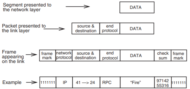
The conceptual model of a network is a cloud bristling with network attachment points identified by numbers known as network addresses, as in Figure \(\PageIndex{1}\) below. A segment enters the network at one attachment point, known as the source. The network layer wraps the segment in a packet and carries the packet across the network to another attachment point, known as the destination, where it unwraps the original segment and delivers it.

The network layer is represented as a large, irregularly shaped cloud (the network) with many short lines (network attachment points) pointing out of the cloud. Each network attachment point is identified by a different number, or network address.

Figure \(\PageIndex{1}\): The network layer.

The model in the figure is misleading in one important way: it suggests that delivery of a segment is accomplished by sending it over one final, physical link. A network attachment point is actually a virtual concept rather than a physical concept. Every network participant, whether a packet forwarder or a client computer system, contains an implementation of the network layer, and when a packet finally reaches the network layer of its destination, rather than forwarding it further, the network layer unwraps the segment contained in the packet and passes that segment to the end-to-end layer inside the system that contains the network attachment point. In addition, a single system may have several network attachment points, each with its own address, all of which result in delivery to the same end-to-end layer; such a system is said to be multihomed. Even packet forwarders need network attachment points with their own addresses, so that a network manager can send them instructions about their configuration and maintenance.

Since a network has many attachment points, the the end-to-end layer must specify to the network layer not only a data segment to transmit but also its intended destination. Further, there may be several available networks and protocols, and several end-to-end protocol handlers, so the interface from the end-to-end layer to the network layer is parallel to the one between the network layer and the link layer:

NETWORK_SEND (segment_buffer, destination, network_protocol, end_layer_protocol)

The argument network_protocol allows the end-to-end layer to select a network and protocol with which to send the current segment, and the argument end_layer_protocol allows for multiplexing, this time of the network layer by the end-to-end layer. The value of end_layer_protocol identifies to the network layer the destination to which end-to-end protocol handler the segment should be delivered.

The network layer also has a link-layer interface, across which it receives packets. Following the upcall style of the link layer of Section 1.4 this interface would be

NETWORK_HANDLE (packet, network_protocol)

and this procedure would be the handler_procedure argument of a call to SET_HANDLER in Figure 1.4.8. Thus whenever the link layer has a packet to deliver to the network layer, it does so by calling NETWORK_HANDLE.

The pseudocode of Figure \(\PageIndex{2}\) describes a model network layer in detail, starting with the structure of a packet, and followed by implementations of the procedures NETWORK_HANDLE and NETWORK_SEND. NETWORK_SEND creates a packet, starting with the segment provided by the end-to-end layer and adding a network-layer header, which here comprises three fields: source , destination , and end_layer_protocol . It fills in the destination and end_layer_protocol fields from the corresponding arguments, and it fills in the source field with the address of its own network attachment point. Figure \(\PageIndex{3}\) shows this latest addition to the overhead of a packet.

Pseudocode for the procedure NETWORK_SEND (which takes the arguments segment_buffer, destination, network_protocol, and end_protocol and sends out packets to other network layers) and the procedure NETWORK_HANDLE (which takes the arguments net_packet and net_protocol, and either forwards received packets to other network layers or passes them to the local end-to-end layer).

Figure \(\PageIndex{2}\): Model implementation of a network layer. The procedure NETWORK_SEND originates packets, while NETWORK_HANDLE receives packets and either forwards them or passes them to the local end-to-end layer.

Procedure NETWORK_HANDLE may do one of two rather different things with a packet, distinguished by the test on line 11. If the packet is not at its destination, NETWORK_HANDLE looks up the packet's destination in forwarding_table to determine the best link on which to forward it, and then it calls the link layer to send the packet on its way. On the other hand, if the received packet is at its destination, the network layer passes its payload up to the end-to-end layer rather than sending the packet out over another link. As in the case of the interface between the link layer and the network layer, the interface to the end-to-end layer is another upcall that is intended to go through a handler dispatcher similar to that of the link layer dispatcher of Figure \(1.4.8\). Because in a network, any network attachment point can send a packet to any other, the last argument of GIVE_TO_END_LAYER, which is the source of the packet, is a piece of information that the end-layer recipient generally finds useful in deciding how to handle the packet.

One might wonder what led to naming the procedure NETWORK_HANDLE rather than NETWORK_RECEIVE. The insight in choosing that name is that forwarding a packet is always done in exactly the same way, whether the packet comes from the layer above or from the layer below. Thus, when we consider the steps to be taken by NETWORK_SEND, the straightforward implementation is simply to place the data in a packet, add a network layer header, and hand the packet to NETWORK_HANDLE. As an extra feature, this architecture allows a source to send a packet to itself without creating a special case.

Just as the link layer used the net_protocol field to decide which of several possible network handlers to give the packet to, NETWORK_SEND can use the net_protocol argument for the same purpose. That is, rather than calling NETWORK_HANDLE directly, it could call the procedure GIVE_TO_NETWORK_HANDLER of Figure \(1.4.8\).

Figure \(\PageIndex{3}\): A typical accumulation of network layer and link layer headers and trailers. The additional information added at each layer can come from control information passed from the higher layer as arguments (for example, the end protocol type and the destination are arguments in the call to the network layer). In other cases they are added by the lower layer (for example, the link layer adds the frame marks and checksum).

Managing the Forwarding Table: Routing

The primary challenge in a packet forwarding network is to set up and manage the forwarding tables, which generally must be different for each network-layer participant. Constructing these tables requires first figuring out appropriate paths (sometimes called routes) to follow from each source to each destination, so the exercise is variously known as path-finding or routing. In a small network, one might set these tables up by hand. As the scale of a network grows, this approach becomes impractical, for several reasons:

The amount of calculation required to determine the best paths grows combinatorially with the number of nodes in the network.
Whenever a link is added or removed, the forwarding tables must be recalculated. As a network grows in size, the frequency of links being added and removed will probably grow in proportion, so the combinatorially growing routing calculation will have to be performed more and more frequently.
Whenever a link fails or is repaired, the forwarding tables must be recalculated. For a given link failure rate, the number of such failures will be proportional to the number of links, so for a second reason the combinatorially growing routing calculation will have to be performed an increasing number of times.
There are usually several possible paths available, and if traffic suddenly causes the originally planned path to become congested, it would be nice if the forwarding tables could automatically adapt to the new situation.

All four of these reasons encourage the development of automatic routing algorithms. If reasons 1 and 2 are the only concerns, one can leave the resulting forwarding tables in place for an indefinite period, a technique known as static routing. The on-the-fly recalculation called for by reasons 3 and 4 is known as adaptive routing, and because this feature is vitally important in many networks, routing algorithms that allow for easy update when things change are almost always used. A packet forwarder that also participates in a routing algorithm is usually called a router. An adaptive routing algorithm requires exchange of current reachability information. Typically, the routers exchange this information using a network-layer routing protocol transmitted over the network itself.

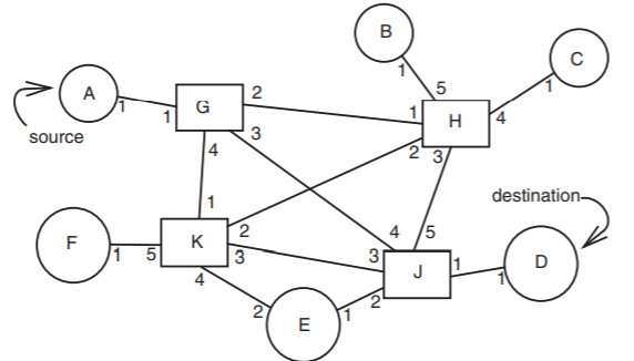
To see how adaptive routing algorithms might work, consider the modest-sized network of Figure \(\PageIndex{4}\). To minimize confusion in interpreting this figure, each network address is lettered, rather than numbered, while each link is assigned two one-digit link identifiers, one from the point of view of each of the stations it connects. In this figure, routers are rectangular while workstations and services are round, but all have network addresses and all have network layer implementations.

Figure \(\PageIndex{4}\): Routing example.

Suppose now that the source \(A\) sends a packet addressed to destination \(D\). Since \(A\) has only one outbound link, its forwarding table is short and simple:

Table \(\PageIndex{1}\): Forwarding table for source A
destination	link
A	end-layer
all other	1

so the packet departs from \(A\) by way of link 1, going to router \(G\) for its next stop. However, the forwarding table at \(G\) must be considerably more complicated. It might contain, for example, the following values:

Table \(\PageIndex{2}\): Forwarding table for router G
destination	link
A	1
B	2
C	2
D	3
E	4
F	4
G	end-layer
H	2
J	3
K	4

This is not the only possible forwarding table for \(G\). Since there are several possible paths to most destinations, there are several possible values for some of the table entries. In addition, it is essential that the forwarding tables in the other routers be coordinated with this forwarding table. If they are not, when router \(G\) sends a packet destined for \(E\) to router \(K\), router \(K\) might send it back to \(G\), and the packet could loop forever.

The interesting question is how to construct a consistent, efficient set of forwarding tables. Many algorithms that sound promising have been proposed and tried; few work well. One that works moderately well for small networks is known as path vector exchange. Each participant maintains, in addition to its forwarding table, a path vector, each element of which is a complete path to some destination. Initially, the only path it knows about is the zero-length path to itself, but as the algorithm proceeds it gradually learns about other paths. Eventually its path vector accumulates paths to every point in the network. After each step of the algorithm it can construct a new forwarding table from its new path vector, so the forwarding table gradually becomes more and more complete. The algorithm involves two steps that every participant repeats over and over, path advertising and path selection.

Table \(\PageIndex{3}\): Initial state of path vector for G. < > is an empty path.
to	path
G	< >

To illustrate the algorithm, suppose participant G starts with a path vector that contains just one item, an entry for itself, as in Table \(\PageIndex{3}\). In the advertising step, each participant sends its own network address and a copy of its path vector down every attached link to its immediate neighbors, specifying the network-layer protocol PATH_EXCHANGE . The routing algorithm of \(G\) would thus receive from its four neighbors the four path vectors of Table \(\PageIndex{4}\). This advertisement allows \(G\) to discover the names, which are in this case network addresses, of each of its neighbors.

Table \(\PageIndex{4}\): Path vectors received by \(G\) in the first round.

From A, via link 1

From H, via link 2

From J, via link 3

From K, via link 4

to	path
A	< >

to	path
H	< >

to	path
J	< >

to	path
K	< >

\(G\) now performs the path selection step by merging the information received from its neighbors with that already in its own previous path vector. To do this merge, \(G\) takes each received path, prepends the network address of the neighbor that supplied it, and then decides whether or not to use this path in its own path vector. Since on the first round in our example all of the information from neighbors gives paths to previously unknown destinations, \(G\) adds all of them to its path vector, as in Table \(\PageIndex{5}\). \(G\) can also now construct a forwarding table for use by NET_HANDLE that allows NET_HANDLE to forward packets to destinations \(A\), \(H\), \(J\), and \(K\) as well as to the end-to-end layer of \(G\) itself. In a similar way, each of the other participants has also constructed a better path vector and forwarding table.

Table \(\PageIndex{5}\): First-round path vector and forwarding table for \(G\).

path vector

forwarding table

to	path
A	<A>
G	<G>
H	<H>
J	<J>
K	<K>

to	link
A	1
G	end-layer
H	2
J	3
K	4

Now, each participant advertises its new path vector. This time, \(G\) receives the four path vectors of Table \(\PageIndex{6}\), which contain information about several participants of which \(G\) was previously unaware. Following the same procedure again, \(G\) prepends to each element of each received path vector the identity of the router that provided it, and then considers whether or not to use this path in its own path vector. For previously unknown destinations, the answer is yes. For previously known destinations, \(G\) compares the paths that its neighbors have provided with the path it already had in its table to see if the neighbor has a better path.

Table \(\PageIndex{6}\): Path vectors received by G in the second round.

From A, via link 1

From H, via link 2:

From J, via link 3:

From K, via link 4:

to	path
A	< >
G	<G>

to	path
B	<B>
C	<C>
G	<G>
H	<H>
J	<J>
K	<K>

to	path
D	<D>
E	<E>
G	<G>
H	<H>
J	<J>
K	<K>

to	path
E	<E>
F	<F>
G	<G>
H	<H>
J	<J>
K	<K>

This comparison raises the question of what metric to use for "better". One simple answer is to count the number of hops. More elaborate schemes might evaluate the data rate of each link along the way or even try to keep track of the load on each link of the path by measuring and reporting queue lengths. Assuming \(G\) is simply counting hops, \(G\) looks at the path that \(A\) has offered to reach \(G\), namely

to G: <A, G>

and notices that \(G\)'s own path vector already contains a zero-length path to \(G\), so it ignores \(A\)'s offering. A second reason to ignore this offering is that its own name, \(G\), is in the path, which means that this path would involve a loop. To ensure loop-free forwarding, the algorithm always ignores any offered path that includes this router's own name. When it is finished with the second round of path selection, \(G\) will have constructed the second-round path vector and forwarding table of Table \(\PageIndex{7}\).

Table \(\PageIndex{7}\): Second-round path vector and forwarding table for \(G\).

path vector

forwarding table

to	path
A	<A>
B	<H, B>
C	<H, C>
D	<J, D>
E	<J, E>
F	<K, F>
G	< >
H	<H>
J	<J>
K	<K>

to	link
A	1
B	2
C	2
D	3
E	3
F	4
G	end-layer
H	2
J	3
K	4

On the next round \(G\) will begin receiving longer paths. For example it will learn that \(H\) offers the path

to D: <H, J, D>

Since this path is longer than the one that \(G\) already has in its own path vector for \(D\), \(G\) will ignore the offer. If the participants continue to alternate advertising and path selection steps, this algorithm ensures that eventually every participant will have in its own path vector the best (in this case, shortest) path to every other participant and there will be no loops.

If static routing would suffice, the path vector construction procedure described above could stop once everyone’s tables had stabilized. But a nice feature of this algorithm is that it is easily extended to provide adaptive routing. One method of extension would be, on learning of a change in topology, to redo the entire procedure, starting again with path vectors containing just the path to the local end layer. A more efficient approach is to use the existing path vectors as a first approximation. The one or two participants who, for example, discover that a link is no longer working simply adjust their own path vectors to stop using that link and then advertise their new path vectors to the neighbors they can still reach. Once we realize that readvertising is a way to adjust to topology change, it is apparent that the straightforward way to achieve adaptive routing is simply to have every router occasionally repeat the path vector exchange algorithm.

If someone adds a new link to the network, on the next iteration of the exchange algorithm, the routers at each end of the new link will discover it and propagate the discovery throughout the network. On the other hand, if a link goes down, an additional step is needed to ensure that paths that traversed that link are discarded: each router discards any paths that a neighbor stops advertising. When a link goes down, the routers on each end of that link stop receiving advertisements; as soon as they notice this lack they discard all paths that went through that link. Those paths will be missing from their own next advertisements, which will cause any neighbors using those paths to discard them in turn; in this way the fact of a down link retraces each path that contains the link, thereby propagating through the network to every router that had a path that traversed the link. A model implementation of all of the parts of this path vector algorithm appears in Figure \(\PageIndex{5}\).

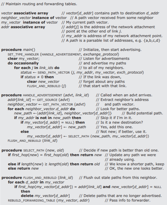
Figure \(\PageIndex{5}\): Model implementation of a path vector exchange routing algorithm. These procedures run in every participating router. They assume that the link layer discards damaged packets. If an advertisement is lost, it is of little consequence because the next advertisement will replace it The procedure REBUILD_FORWARDING_TABLE is not shown; it simply constructs a new forwarding table for use by this router, using the latest path vector information.

When designing a routing algorithm, there are a number of questions that one should ask. Does the algorithm converge? (Because it selects the shortest path this algorithm will converge, assuming that the topology remains constant.) How rapidly does it converge? (If the shortest path from a router to some participant is \(N\) steps, then this algorithm will insert that shortest path in that router's table after \(N\) advertising/path-selection exchanges.) Does it respond equally well to link deletions? (No, it can take longer to convince all participants of deletions. On the other hand, there are other algorithms—such as distance vector, which passes around just the lengths of paths rather than the paths themselves—that are much worse.) Is it safe to send traffic before the algorithm converges? (If a link has gone down, some packets may loop for a while until everyone agrees on the new forwarding tables. This problem is serious, but in the next paragraph we will see how to fix it by discarding packets that have been forwarded too many times.) How many destinations can it reasonably handle? (The Border Gateway Protocol, which uses a path vector algorithm similar to the one described above, has been used in the Internet to exchange information concerning 100,000 or so routes.)

The possibility of temporary loops in the forwarding tables or more general routing table inconsistencies, buggy routing algorithms, or misconfigurations can be dealt with by a network layer mechanism known as the hop limit. The idea is to add a field to the network-layer header containing a hop limit counter. The originator of the packet initializes the hop limit. Each router that handles the packet decrements the hop limit by one as the packet goes by. If a router finds that the resulting value is zero, it discards the packet. The hop limit is thus a safety net that ensures that no packet continues bouncing around the network forever.

There are some obvious refinements that can be made to the path vector algorithm. For example, since nodes such as \(A\), \(B\), \(C\), \(D\), and \(F\) are connected by only one link to the rest of the network, they can skip the path selection step and just assume that all destinations are reachable via their one link—but when they first join the network they must do an advertising step, to ensure that the rest of the network knows how to reach them (and it would be wise to occasionally repeat the advertising step, to make sure that link failures and router restarts don’t cause them to be forgotten). A service node such as \(E\), which has two links to the network but is not intended to be used for transit traffic, may decide never to advertise anything more than the path to itself. Because each participant can independently decide which paths it advertises, path vector exchange is sometimes used to implement restrictive routing policies. For example, a country might decide that packets that both originate and terminate domestically should not be allowed to transit another country, even if that country advertises a shorter path.

The exchange of data among routers is just another example of a network layer protocol. Since the link layer already provides network layer protocol multiplexing, no extra effort is needed to add a routing protocol to the layered system. Further, there is nothing preventing different groups of routers from choosing to use different routing protocols among themselves. In the Internet, there are many different routing protocols simultaneously in use, and it is common for a single router to use different routing protocols over different links.

Hierarchical Address Assignment and Hierarchical Routing

The system for identifying attachment points of a network as described so far is workable, but does not scale up well to large numbers of attachment points. There are two immediate problems:

Every attachment point must have a unique address. If there are just ten attachment points, all located in the same room, coming up with a unique identifier for an eleventh is not difficult. But if there are several hundred million attachment points in locations around the world, as in the Internet, it is hard to maintain a complete and accurate list of addresses already assigned.
The path vector grows in size with the number of attachment points. Again, for routers to exchange a path vector with ten entries is not a problem; a path vector with 100 million entries could be a hassle.

The usual way to tackle these two problems is to introduce hierarchy: invent some scheme by which network addresses have a hierarchical structure that we can take advantage of, both for decentralizing address assignments and for reducing the size of forwarding tables and path vectors.

For example, consider again the abstract network of Figure \(\PageIndex{1}\), in which we arbitrarily assigned two-digit numbers as network addresses. Suppose we instead adopt a more structured network address consisting, say, of two parts, which we might call "region" and "station". Thus in Figure \(\PageIndex{4}\) we might assign to A the network address "11,75" where 11 is a region identifier and 75 is a station identifier.

By itself, this change merely complicates things. However, if we also adopt a policy that regions must correspond to the set of network attachment points served by an identifiable group of closely-connected routers, we have a lever that we can use to reduce the size of forwarding tables and path vectors. Whenever a router for region 11 gets ready to advertise its path vector to a router that serves region 12, it can condense all of the paths for the region 11 network destinations it knows about into a single path, and simply advertise that it knows how to forward things to any region 11 network destination. The routers that serve region 11 must, of course, still maintain complete path vectors for every region 11 station, and exchange those vectors among themselves, but these vectors are now proportional in size to the number of attachment points in region 11, rather than to the number of attachment points in the whole network.

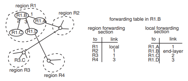
When a network uses hierarchical addresses, the operation of forwarding involves the same steps as before, but the table lookup process is slightly more complicated: The forwarder must first extract the region component of the destination address and look that up in its forwarding table. This lookup has two possible outcomes: either the forwarding table contains an entry showing a link over which to send the packet to that region, or the forwarding table contains an entry saying that this forwarder is already in the destination region, in which case it is necessary to extract the station identifier from the destination address and look that up in a distinct part of the forwarding table. In most implementations, the structure of the forwarding table reflects the hierarchical structure of network addresses. Figure \(\PageIndex{6}\) illustrates the use of a forwarding table for hierarchical addresses that is constructed of two sections.

Figure \(\PageIndex{6}\): Example of a forwarding table with regional addressing in network node R1.B. The forwarder first looks up the region identifier in the region forwarding section of the table. If the target address is R3.C, the region identifier is R3, so the table tells it that it should forward the packet on link 1. If the target address is R1.C, which is in its own region R1, the region forwarding table tells it that R1 is the local region, so it then looks up R1.C in the local forwarding section of the table. There may be hundreds of network attachment points in region R3, but just one entry is needed in the forwarding table at node R1.B.

Hierarchical addresses also offer an opportunity to grapple with the problem of assigning unique addresses in a large network because the station part of a network address needs to be unique only within its region. A central authority can assign region identifiers, while different local authorities can assign the station identifiers within each region, without consulting other regional authorities. For this decentralization to work, the boundaries of each local administrative authority must coincide with the boundaries of the regions served by the packet forwarders. While this seems like a simple thing to arrange, it can actually be problematic. One easy way to define regions of closely connected packet forwarders is to do it geographically. However, administrative authority is often not organized on a strictly geographic basis. So there may be a significant tension between the needs of address assignment and the needs of packet forwarding.

Hierarchical network addresses are not a panacea—in addition to complexity, they introduce at least two new problems. With the non-hierarchical scheme, the geographical location of a network attachment point did not matter, so a portable computer could, for example, connect to the network in either Boston or San Francisco, announce its network address, and after the routers have exchanged path vectors a few times, expect to communicate with its peers. But with hierarchical routing, this feature stops working. When a portable computer attaches to the network in a different region, it cannot simply advertise the same network address that it had in its old region. It will instead have to first acquire a network address within the region to which it is attaching. In addition, unless some provision has been made at the old address for forwarding, other stations in the network that remember the old network address will find that they receive no-answer responses when they try to contact this station, even though it is again attached to the network.

The second complication is that paths may no longer be the shortest possible because the path vector algorithm is working with less detailed information. If there are two different routers in region 5 that have paths leading to region 7, the algorithm will choose the path to the nearest of those two routers, even though the other router may be much closer to the actual destination inside region 7.

We have used in this example a network address with two hierarchical levels, but the same principle can be extended to as many levels as are needed to manage the network. In fact, any region can do hierarchical addressing within just the part of the address space that it controls, so the number of hierarchical levels can be different in different places. The public Internet uses just two hierarchical addressing levels, but some large subnetworks of the Internet implement the second level internally as a two-level hierarchy. Similarly, North American telephone providers have created a four-level hierarchy for telephone numbers: country code, area code, exchange, and line number, for exactly the same reasons: to reduce the size of the tables used in routing calls, and to allow local administration of line numbers. Other countries agree on the country codes but internally may have a different number of hierarchical levels.

Reporting Network Layer Errors

The network layer can encounter trouble when trying to forward a packet, so it needs a way of reporting that trouble. The network layer is in a uniquely awkward position when this happens because the usual reporting method (return a status value to the higher-layer program that asked for this operation) may not be available. An intermediate router receives a packet from a link layer below, and it is expected to forward that packet via another link layer. Even if there is a higher layer in the router, that layer probably has no interest in this packet. Instead, the entity that needs to hear about the problem is more likely to be the upper layer program that originated the packet, and that program may be located several hops away in another computer. Even the network layer at the destination address may need to report something to the original sender such as the lack of an upper-layer handler for the end-to-end type that the sender specified.

The obvious thing to do is send a message to the entity that needs to know about the problem. The usual method is that the network layer of the router creates a new packet on the spot and sends it back to the source address shown in the problem packet. The message in this new packet reports details of the problem using some standard error reporting protocol. With this design, the original higher-layer sender of a packet is expected to listen not only for replies but also for messages of the error reporting protocol. Here are some typical error reports:

The buffers of the router were full, so the packet had to be discarded.
The buffers of the router are getting full—please stop sending so many packets.
The region identifier part of the target address does not exist.
The station identifier part of the target address does not exist.
The end type identifier was not recognized.
The packet is larger than the maximum transmission unit of the next link.
The packet hop limit has been exceeded.

In addition, a copy of the header of the doomed packet goes into a data field of the error message, so that the recipient can match it with an outstanding SEND request.

One might suggest that a router send an error report when discarding a packet that is received with a wrong checksum. This idea is not as good as it sounds because a damaged packet may have garbled header information, in which case the error message might be sent to a wrong—or even nonexistent—place. Once a packet has been identified as containing unknown damage, it is not a good idea to take any action that depends on its contents.

A network-layer error reporting protocol is a bit unusual. An error message originates in the network layer, but is delivered to the end-to-end layer. Since it crosses layers, it can be seen as violating (in a minor way) the usual separation of layers: we have a network layer program preparing an end-to-end header and inserting end-to-end data; a strict layer doctrine would insist that the network layer not touch anything but network layer headers.

An error reporting protocol is usually specified to be a best-effort protocol, rather than one that takes heroic efforts to get the message through. There are two reasons why this design decision makes sense. First, as will be seen in Section 1.6, implementing a more reliable protocol adds a fair amount of machinery: timers, keeping copies of messages in case they need to be retransmitted, and watching for receipt acknowledgments. The network layer is not usually equipped to do any of these functions, and not implementing them minimizes the violation of layer separation. Second, error messages can be thought of as hints that allow the originator of a packet to more quickly discover a problem. If an error message gets lost, the originator should, one way or another, eventually discover the problem in some other way, perhaps after timing out, resending the original packet, and getting an error message on the retry.

A good example of the best-effort nature of an error reporting protocol is that it is common to not send an error message about every discarded packet; if congestion is causing the discard rate to climb, that is exactly the wrong time to increase the network load by sending many “I discarded your packet” notices. But sending a few such notices can help alert sources who are flooding the network that they need to back off—this topic is explored in more depth in Section 1.7.

The basic idea of an error reporting protocol can be used for other communications to and from the network layer of any participant in the network. For example, the Internet has a protocol named internet control message protocol (ICMP) that includes an echo request message (also known as a "ping," from an analogy with submarine active sonar systems). If an end node sends an echo request to any network participant, whether a packet forwarder or another end node, the network layer in that participant is expected to respond by immediately sending the data of the message back to the sender in an echo reply message. Echo request/reply messages are widely used to determine whether or not a participant is actually up and running. They are also sometimes used to assess network congestion by measuring the time until the reply comes back.

Another useful network error report is "hop limit exceeded". Recall from Section 1.5.2 that to provide a safety net against the possibility of forwarding loops, a packet may contain a hop limit field, which a router decrements in each packet that it forwards. If a router finds that the hop limit field contains zero, it discards the packet and it also sends back a message containing the error report. The "hop limit exceeded" error message provides feedback to the originator, for example it may have chosen a hop limit that is too small for the network configuration. The "hop limit exceeded" error message can also be used in an interesting way to help locate network problems: send a test message (usually called a probe) to some distant destination address, but with the hop limit set to 1. This probe will cause the first router that sees it to send back a “hop limit exceeded” message whose source address identifies that first router. Repeat the experiment, sending probes with hop limits set to 2, 3,…, etc. Each response will reveal the network address of the next router along the current path between the source and the destination. In addition, the time required for the response to return gives a rough indication of the network load between the source and that router. In this way one can trace the current path through the network to the destination address, and identify points of congestion.

Another way to use an error reporting protocol is for the end-to-end layer to send a series of probes to learn the smallest maximum transmission unit (MTU) that lies on the current path between it and another network attachment point. It first sends a packet of the largest size the application has in mind. If this probe results in an "MTU exceeded" error response, it halves the packet size and tries again. A continued binary search will quickly home in on the smallest MTU along the path. This procedure is known as MTU discovery.

Network Address Translation (An Idea That Almost Works)

From a naming point of view, the Internet provides a layered naming environment with two contexts for its network attachment points, known as "Internet addresses". An Internet address has two components, a network number and a host number. Most network numbers are global names, but a few, such as network 10, are designated for use in private networks. These network numbers can be used either completely privately, or in conjunction with the public Internet. Completely private use involves setting up an independent private network, and assigning host addresses using the network number 10. Routers within this network advertise and forward just as in the public Internet. Routers on the public Internet follow the convention that they do not accept routes to network 10, so if this private network is also directly attached to the public Internet, there is no confusion. Assuming that the private network accepts routes to globally named networks, a host inside the private network could send a message to a host on the public Internet, but a host on the public Internet cannot send a response back because of the routing convention. Thus any number of private networks can each independently assign numbers using network number 10—but hosts on different private networks cannot talk to one another and hosts on the public Internet cannot talk to them.

Network Address Translation (NAT) is a scheme to bridge this gap. The idea is that a specialized translating router (known informally as a "NAT box") stands at the border between a private network and the public Internet. When a host inside the private network wishes to communicate with a service on the public Internet, it first makes a request to the translating router. The translator sets up a binding between that host’s private address and a temporarily assigned public address, which the translator advertises to the public Internet. The private host then launches a packet that has a destination address in the public Internet, and its own private network source address. As this packet passes through the translating router, the translator modifies the source address by replacing it with the temporarily assigned public address. It then sends the packet on its way into the public Internet. When a response from the service on the public Internet comes back to the translating router, the translator extracts the destination address from the response, looks it up in its table of temporarily assigned public addresses, finds the internal address to which it corresponds, modifies the destination address in the packet, and sends the packet on its way on the internal network, where it finds its way to the private host that initiated the communication.

The scheme works, after a fashion, but it has a number of limitations. The most severe limitation is that some end-to-end network protocols place Internet addresses in fields buried in their payloads; there is nothing restricting Internet addresses to packet source and destination fields of the network layer header. For example, some protocols between two parties start by mentioning the Internet address of a third party, such as a bank, that must also participate in the protocol. If the Internet address of the third party is on the public Internet, there may be no problem, but if it is an address on the private network, the translator needs to translate it as it goes by. The trouble is that translation requires that the translator peer into the payload data of the packet and understand the format of the higher-layer protocol. The result is that NAT works only for those protocols that the translator is programmed to understand. Some protocols may present great difficulties. For example, if a secure protocol uses key-driven cryptographic transformations for either privacy or authentication, the NAT gateway would need to have a copy of the keys, but giving it the keys may defeat the purpose of the secure protocol. (This concern will become clearer after reading Chapter 5.

A second problem is that all of the packets between the public Internet and the private network must pass through the translating router, since it is the only place that knows how to do the address translation. The translator thus introduces both a potential bottleneck and a potential single point of failure, and NAT becomes a constraint on routing policy.

A third problem arises if two such organizations later merge. Each organization will have assigned addresses in network 10, but since their assignments were not coordinated, some addresses will probably have been assigned in both organizations, and all of the colliding addresses must be discovered and changed.

Although originally devised as a scheme to interconnect private networks to the public Internet, NAT has become popular as a technique to beef up security of computer systems that have insecure operating system or network implementations. In this application, the NAT translator inspects every packet coming from the public Internet and refuses to pass along any whose origin seems suspicious or that try to invoke services that are not intended for public use. The scheme does not in itself provide much security, but in conjunction with other security mechanisms described in Chapter 5, it can help create what that chapter describes as "defense in depth".