7.2: Probability Diagrams

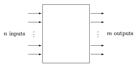
The probability model of a process with \(n\) inputs and \(m\) outputs, where \(n\) and \(m\) are integers, is shown in Figure 7.5. The \(n\) input states are mutually exclusive, as are the \(m\) output states. If this process is implemented by logic gates the input would need at least \(\log_2(n)\) but not as many as \(n\) wires.

Figure 7.3: Probability model of a two-input one-output gate.

Figure 7.4: Probability model of an \(AND\) gate

This model for processes is conceptually simple and general. It works well for processes with a small number of bits. It was used for the binary channel in Chapter 6.

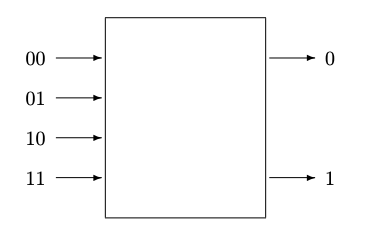
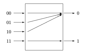
Unfortunately, the probability model is awkward when the number of input bits is moderate or large. The reason is that the inputs and outputs are represented in terms of mutually exclusive sets of events. If the events describe signals on, say, five wires, each of which can carry a high or low voltage signifying a boolean 1 or 0, there would be 32 possible events. It is much easier to draw a logic gate, with five inputs representing physical variables, than a probability process with 32 input states. This “exponential explosion” of the number of possible input states gets even more severe when the process represents the evolution of the state of a physical system with a large number of atoms. For example, the number of molecules in a mole of gas is Avogadro’s number \(N_A = 6.02 × 10^{23}\). If each atom had just one associated boolean variable, there would be 2\(^{N_A}\) states, far greater than the number of particles in the universe. And there would not be time to even list all the particles, much less do any calculations: the number of microseconds since the big bang is less than 5 × 10\(^{23}\). Despite this limitation, the probability diagram model is useful conceptually.

Let’s review the fundamental ideas in communications, introduced in Chapter 6, in the context of such diagrams.

We assume that each possible input state of a process can lead to one or more output state. For each

Figure 7.5: Probability model

input \(i\) denote the probability that this input leads to the output \(j\) as \(c_{ji}\). These transition probabilities \(c_{ji}\) can be thought of as a table, or matrix, with as many columns as there are input states, and as many rows as output states. We will use \(i\) as an index over the input states and \(j\) over the output states, and denote the event associated with the selection of input \(i\) as \(A_i\) and the event associated with output \(j\) as \(B_j\).

The transition probabilities are properties of the process, and do not depend on the inputs to the process. The transition probabilities lie between 0 and 1, and for each \(i\) their sum over the output index \(j\) is 1, since for each possible input event exactly one output event happens. If the number of input states is the same as the number of output states then \(c_{ji}\) is a square matrix; otherwise it has more columns than rows or vice versa.

\(0 \leq c_{ji} \leq 1 \tag{7.1}\)

\(1 = \displaystyle \sum_{j} c_{ji} \tag{7.2}\)

This description has great generality. It applies to a deterministic process (although it may not be the most convenient—a truth table giving the output for each of the inputs is usually simpler to think about). For such a process, each column of the \(c_{ji}\) matrix contains one element that is 1 and all the other elements are 0. It also applies to a nondeterministic channel (i.e., one with noise). It applies to the source encoder and decoder, to the compressor and expander, and to the channel encoder and decoder. It applies to logic gates and to devices which perform arbitrary memoryless computation (sometimes called “combinational logic” in distinction to “sequential logic” which can involve prior states). It even applies to transitions taken by a physical system from one of its states to the next. It applies if the number of output states is greater than the number of input states (for example channel encoders) or less (for example channel decoders).

If a process input is determined by random events \(A_i\) with probability distribution \(p(A_i)\) then the various other probabilities can be calculated. The conditional output probabilities, conditioned on the input, are

\(p(B_j \; |\; A_i) = c_{ji} \tag{7.3}\)

The unconditional probability of each output \(p(B_j)\) is

\(p(B_j = \displaystyle \sum_{i} c_{ji}p(A_i) \tag{7.4}\)

Finally, the joint probability of each input with each output \(p(A_i, B_j)\) and the backward conditional probabilities \(p(A_i \;|\; B_j)\) can be found using Bayes’ Theorem:

\[\begin{align*} p(A_i, B_j) & = p(B_j)p(A_i \;|\; B_j) \tag{7.5} \\ & = p(A_i)p(B_j \;|\; A_i) \tag{7.6} \\ & = p(A_i)c_{ji} \tag{7.7} \end{align*} \]