7.7: Cascaded Processes

Consider two processes in cascade. This term refers to having the output from one process serve as the input to another process. Then the two cascaded processes can be modeled as one larger process, if the “internal” states are hidden. We have seen that discrete memoryless processes are characterized by values of \(I\), \(J\), \(L\), \(N\), and \(M\). Figure 7.10(a) shows a cascaded pair of processes, each characterized by its own parameters. Of course the parameters of the second process depend on the input probabilities it encounters, which are determined by the transition probabilities (and input probabilities) of the first process.

But the cascade of the two processes is itself a discrete memoryless process and therefore should have its own five parameters, as suggested in Figure 7.10(b). The parameters of the overall model can be calculated

(a) The two processes

(b) Equivalent single process

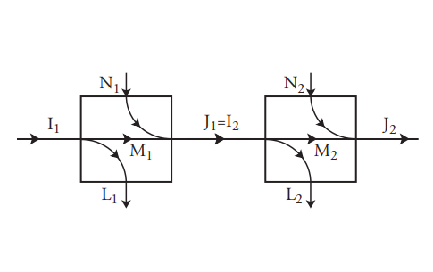
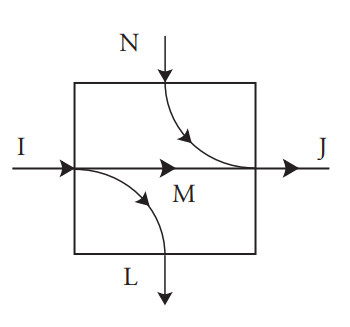
Figure 7.10: Cascade of two discrete memoryless processes

either of two ways. First, the transition probabilities of the overall process can be found from the transition probabilities of the two models that are connected together; in fact the matrix of transition probabilities is merely the matrix product of the two transition probability matrices for process 1 and process 2. All the parameters can be calculated from this matrix and the input probabilities.

The other approach is to seek formulas for \(I\), \(J\), \(L\), \(N\), and \(M\) of the overall process in terms of the corresponding quantities for the component processes. This is trivial for the input and output quantities: \(I = I_1\) and \(J = J_2\). However, it is more difficult for \(L\) and \(N\). Even though \(L\) and \(N\) cannot generally be found exactly from \(L_1\), \(L_2\), \(N_1\) and \(N_2\), it is possible to find upper and lower bounds for them. These are useful in providing insight into the operation of the cascade.

It can be easily shown that since \(I = I_1\), \(J_1 = I_2\), and \(J = J_2\),

\(L − N = (L_1 + L_2) − (N_1 + N_2) \tag{7.33}\)

It is then straightforward (though perhaps tedious) to show that the loss \(L\) for the overall process is not always equal to the sum of the losses for the two components \(L_1 + L_2\), but instead

\(0 ≤ L_1 ≤ L ≤ L_1 + L_2 \tag{7.34}\)

so that the loss is bounded from above and below. Also,

\(L_1 + L_2 − N_1 ≤ L ≤ L_1 + L_2 \tag{7.35}\)

so that if the first process is noise-free then \(L\) is exactly \(L_1 + L_2\).

There are similar formulas for \(N\) in terms of \(N_1 + N_2\):

\(0 ≤ N_2 ≤ N ≤ N_1 + N_2 \tag{7.36}\)

\(N_1 + N_2 − L_2 ≤ N ≤ N_1 + N_2 \tag{7.37}\)

Similar formulas for the mutual information of the cascade \(M\) follow from these results:

\(M_1 − L_2 ≤ M ≤ M_1 ≤ I \tag{7.38}\)

\(M_1 − L_2 ≤ M ≤ M_1 + N_1 − L_2 \tag{7.39}\)

\(M_2 − N_1 ≤ M ≤ M_2 ≤ J \tag{7.40}\)

\(M_2 − N_1 ≤ M ≤ M_2 + L_2 − N_1 \tag{7.41}\)

Other formulas for \(M\) are easily derived from Equation 7.19 applied to the first process and the cascade, and Equation 7.24 applied to the second process and the cascade:

\(\begin{align*} M &= M_1 + L_1 − L \\ &= M_1 + N_1 + N_2 − N − L_2 \\ &= M_2 + N_2 − N \\ &= M_2 + L_2 + L_1 − L − N_1 \tag{7.42} \end{align*}\)

where the second formula in each case comes from the use of Equation 7.33. Note that \(M\) cannot exceed either \(M_1\) or \(M_2\), i.e., \(M ≤ M_1\) and \(M ≤ M_2\). This is consistent with the interpretation of \(M\) as the information that gets through—information that gets through the cascade must be able to get through the first process and also through the second process.

As a special case, if the second process is lossless, \(L_2 = 0\) and then \(M = M_1\). In that case, the second process does not lower the mutual information below that of the first process. Similarly if the first process is noiseless, then \(N_1 = 0\) and \(M = M_2\).

The channel capacity \(C\) of the cascade is, similarly, no greater than either the channel capacity of the first process or that of the second process: \(C ≤ C_1\) and \(C ≤ C_2\). Other results relating the channel capacities are not a trivial consequence of the formulas above because \(C\) is by definition the maximum \(M\) over all possible input probability distributions—the distribution that maximizes \(M_1\) may not lead to the probability distribution for the input of the second process that maximizes \(M_2\).