17.2: Well Posedness

We will restrict attention to the feedback structure in Figure 17.5. Our assumption is that \(H_{1}\) and \(H_{2}\) have some underlying state-space descriptions with inputs \(u_{1}\), \(u_{2}\) and outputs \(y_{1}\), \(y_{2}\), so their transfer functions \(H_{1}(s)\) and \(H_{2}(s)\) are proper, i.e. \(H_{1}(\infty)\), \(H_{2}(\infty)\) are finite. It is possible (and in fact typical for models of physical systems, since their response falls off to zero as one goes higher in frequency) that the transfer function is in fact strictly proper.

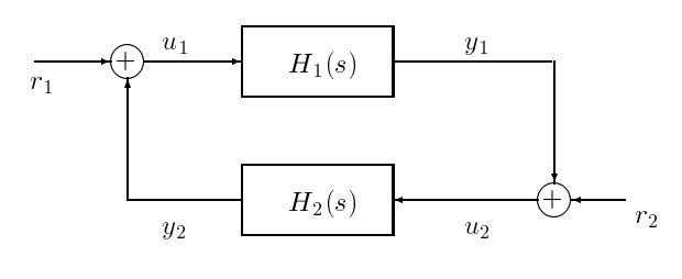
Figure \(\PageIndex{1}\): Feedback Interconnection

The closed-loop system in Figure 17.3.5 can now be described in state-space form by writing down state-space descriptions for \(H_{1}(s)\) (with input \(u_{1}\) and output \(y_{1}\)) and \(H_{2}(s)\) (with input \(u_{2}\) and output \(y_{2}\)), and combining them according to the interconnection constraints represented in Figure 17.3.5. Suppose our state-space models for \(H_{1}\) and \(H_{2}\) are

\[H_{1} \sim\left[\begin{array}{cc}
A_{1} & B_{1} \\
C_{1} & D_{1}
\end{array}\right], \quad H_{2} \sim\left[\begin{array}{cc}
A_{2} & B_{2} \\
C_{2} & D_{2}
\end{array}\right]\nonumber\]

with respective state vectors, inputs, and outputs \(\left(x_{1}, u_{1}, y_{1}\right)\) and \(\left(x_{2}, u_{2}, y_{2}\right)\), so

\[\begin{aligned}
\dot{x}_{1} &=A_{1} x_{1}+B_{1} u_{1} \\
y_{1} &=C_{1} x_{1}+D_{1} u_{1} \\
\dot{x}_{2} &=A_{2} x_{2}+B_{2} u_{2} \\
y_{2} &=C_{2} x_{2}+D_{2} u_{2}
\end{aligned} \ \tag{17.1}\]

Note that \(D_{1}=H_{1}(\infty)\) and \(D_{2}=H_{2}(\infty)\). The interconnection constraints are embodied in the following set of equations:

\[\begin{array}{l}
u_{1}=r_{1}+y_{2}=r_{1}+C_{2} x_{2}+D_{2} u_{2} \\
u_{2}=r_{2}+y_{1}=r_{2}+C_{1} x_{1}+D_{1} u_{1},
\end{array}\nonumber\]

which can be rewritten compactly as

\[\left[\begin{array}{cc}
I & -D_{2} \\
-D_{1} & I
\end{array}\right]\left[\begin{array}{l}
u_{1} \\
u_{2}
\end{array}\right]=\left[\begin{array}{cc}
0 & C_{2} \\
C_{1} & 0
\end{array}\right]\left[\begin{array}{l}
x_{1} \\
x_{2}
\end{array}\right]+\left[\begin{array}{cc}
I & 0 \\
0 & I
\end{array}\right]\left[\begin{array}{l}
r_{1} \\
r_{2}
\end{array}\right] \ \tag{17.2}\]

We shall label the interconnected system well-posed if the internal signals of the feed- back loop, namely \(u_{1}\) and \(u_{2}\), are uniquely defined for every choice of the system state variables \(x_{1}\), \(x_{2}\) and external inputs \(r_{1}\), \(r_{2}\). (Note that the other internal signals, \(y_{1}\) and \(y_{2}\), will be uniquely defined under these conditions if and only if \(u_{1}\) and \(u_{2}\) are, so we just focus on the latter pair.) It is evident from (17.2) that the condition for this is the invertibility of the matrix

\[\left[\begin{array}{cc}
I & -D_{2} \\
-D_{1} & I
\end{array}\right] \ \tag{17.3}\]

This matrix is invertible if and only if

\[I-D_{1} D_{2} \text{ or equivalently } I-D_{2} D_{1} \text{ is invertible } \ \tag{17.4}\]

This result follows from the fact that if \(X\), \(Y\), \(W\) and \(Z\) are matrices of compatible dimensions, and \(X\) is invertible then

\[\operatorname{det}\left[\begin{array}{cc}
X & Y \\
Z & W
\end{array}\right]=\operatorname{det}(X) \operatorname{det}\left(W-Z X^{-1} Y\right) \ \tag{17.5}\]

A sufficient condition for (17.4) to hold is that either \(H_{1}\) or \(H_{2}\) (or both) be strictly proper; that is, either \(D_{1} = 0\) or \(D_{2} = 0\).

The significance of well-posedness is that once we have solved (17.2) to determine \(u_{1}\) and \(u_{2}\) in terms of \(x_{1}\), \(x_{2}\), \(r_{1}\) and \(r_{2}\), we can eliminate \(u_{1}\) and \(u_{2}\) from (17.1) and arrive at a state-space description of the closed-loop system, with state vector

\[x=\left(\begin{array}{l}
x_{1} \\
x_{2}
\end{array}\right)\nonumber\]

We leave you to write down this description explicitly. Without well-posedness, \(u_{1}\) and \(u_{2}\) would not be well-defined for arbitrary \(x_{1}\), \(x_{2}\), \(r_{1}\) and \(r_{2}\), which would in turn mean that there could not be a well-defined state-space representation of the closed-loop system.

The condition in (17.4) is equivalent to requiring that

\[\left(I-H_{1}(s) H_{2}(s)\right)^{-1} \text{ or equivalently } \left(I-H_{1}(s) H_{2}(s)\right)^{-1} \text{ exists and is proper } \ \tag{17.6}\]

Example 17.1

Consider a discrete-time system with \(H_{1}(z) = 1\) and \(H_{2}(z) = 1- z^{-1}\) in (the DT version of ) Figure 17.5. In this case \(\left(1-H_{1}(\infty) H_{2}(\infty)\right)=1-1=0\), and thus the system is ill-posed. Note that the transfer function from \(r_{1}\) to \(y_{1}\) for this system is

\[\left(1-H_{1} H_{2}\right)^{-1} H_{1}=\left(1-1+z^{-1}\right)^{-1}=z\nonumber\]

which is not proper - it actually corresponds to the noncausal input-output relation

\[y_{1}(k)=r_{1}(k+1)\nonumber\]

which cannot be modeled by a state-space description.

Example 17.2

Again consider Figure 17.4, with \(H_{1}(s)=\frac{s+1}{s+2}\) and \(H_{2}(s)=\frac{s+2}{s+1}\) The expression \(\left(1-H_{1}(\infty) H_{2}(\infty)\right)=0\), which implies that the interconnection is ill-posed. In this case notice that,

\[\begin{aligned}
\left(1-H_{1}(s) H_{2}(s)\right) &=1-1 \\
&=0 \quad \forall s \in \mathbb{C} \ !
\end{aligned}\nonumber\]

Since the inverse of \((1 - H_{1}H_{2})\) does not exist, the transfer functions relating external signals to internal signals cannot be written down.