Chapter 3: Polymer Chain Models

Polymer Chain Conformations

We now know how to create polymers and we have discussed some of the unique characteristics of polymer chains (inter vs intramolecular bonding). We also have seen some of the different polymer architectures that we will encounter but we haven’t really talked much about polymer conformations. I make a distinction here between architecture and conformation. Polymer architecture has a connotation referring to the the structure of the polymer whereas a polymer chain conformation has a connotation which refers to the instantaneous state of the polymer especially when subjected to an external stimuli.

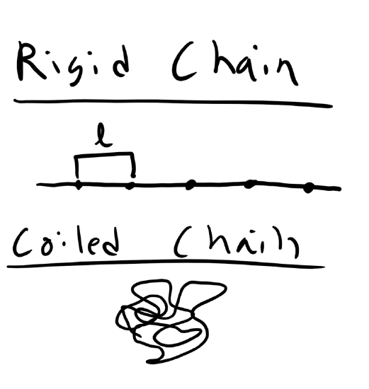
In our discussion of polymer chain conformations we will start simple and build up from a simple homopolymer with a very high molecular weight. So this polymer architecture is simply linear, flexible, chain or if you like macroscopic analogies spaghetti. And the flexibility of the chain will be governed by the intramolecular bonding of the repeat unit, as well as other factors which we will get into in depth when we discuss the glass transition temperature. One of the key ways that we can characterize a polymer chain conformation, just like we did with molar mass in the previous lecture, is by describing the effective size of a single polymer chain in solution. Now you might reasonably think that the size of a linear polymer chain is simply the length of the monomer or repeat unit multiplied by the number of repeat units. However, this is not the case as we are interested in the effective size of the polymer which is the space occupied by the polymer. We will see in this lecture that depending on the temperature, solvent, and local environment even this simple polymer chain can adopted a highly coiled collapsed structure, an highly elongated structure, or even in the most extreme circumstances a fully elongated structure. We also know from our supplemental thermodynamics notes that polymers can adopt a large number of possible conformation, microstates. The conformation and thus the effective size of the polymer can change rapidly. This means that we will also have to develop a metric to measure the size of the polymer which is probabilistic in nature.

You can see this in the embedded video in the PowerPoint slides.

We will describe in detail several different models which will describe the effective size of polymers with increasing complexity

• Ideal/Freely Jointed Chain Model
• Mathematician’s Ideal Chain
• Chemist’s Chain in Solution and Melt Model
• Physicist’s Ideal Chain

We will examine the differences in each model and how the scaling changes depending on some of the factors mentioned above.

Characterizing Polymer Size: Mean-Squared-Displacement

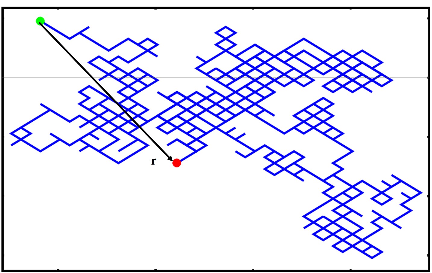
We have just mentioned that describing the effective size of the polymer can be tricky and it is not just a matter of adding up the monomer lengths. This problem becomes even more complex when we are dealing with polymers with a more complex architecture, i.e. branched, dendrimer, star polymers, syndiotactic, etc. How do we characterize the size of a polymer then? Well the tool that we will use is the root mean squared end to end distance (RMSD) which is shown below

$$\langle r^{2} \rangle^{\frac{1}{2}} \nonumber$$

where r is the vectorial position of the polymer at one end and the other end in 3D, seen in the image below

We take the square because this will give us a quantity in units of length. Note as well that the this indicates an average quantity as we will typically average over many microstates and conformations. You can also see that by squaring the r we will never have negative values. Now there are many ways of calculating a mean square displacement. One method is simply averaging the end-to-end displacement values of a single polymer chain as it moves and fluctuates over time or you can average one snapshot of identical polymer chains which are all under the same external stimuli/experimental conditions.

To get started let’s do a quick couple of extreme example of a linear rigid rod like polymer architecture that is stretched to the fully extended position. This polymer has a monomer length of l and the number of monomers is as always n. What is the MSD end-to-end distance?

Well let’s start with the r vector?

It is nl! So

$$\langle r^2 \rangle^{\frac{1}{2}} = nl = L \nonumber$$

where L is the contour length of the polymer, the fully extended distance.

Ideal/Freely Jointed Chain (FJC)/Gaussian Model

Now the above example is an very extreme situation, although an important one to consider. However, polymers are not typically fully extended and this is an energetically unfavorable microstate. To describe a more typical polymer conformation let’s start with a simpler model. Let’s consider an ideal polymer chain where we assume that there are no intramolecular steric interactions along the polymer chain. This means that the polymer can intersect itself along the backbone without any penalty. This is the Ideal/FJC/Gaussian Chain Model.

So again here we have a polymer chain with a monomer length, l, and a number of monomers, n. We also assume that in addition to the ability of chain to cross over itself the monomers can rotate in any dimension with respect to one another. We are essentially ignoring the constraints that double or triple carbon bonds can place on polymer rotation, steric or repulsive interactions, or intermolecular interactions. So with all of these assumptions we can describe the polymer as essentially performing a random walk through space in time. Or alternatively we can construct a polymer chain by placing each monomer in a position in space using a stochastic or random algorithm (Monte Carlo). In this random walk the step size would be fixed at l from the previous step/monomer and would continue until reaching n random steps. Thus the position of monomer i and i + 1 are completely uncorrelated.

Let's start building our polymer chain taking a probabilistic approach in 1D. In 1D we can only move left or right and we will indicate that steps to the right are positive $+$ and the left steps are negative $-$. So our $r$ vector will simply be:

$$r = (n_{+} - n_{-})l \nonumber$$

where $n_+$ is the number of right/positive steps and $n_-$ is the number of left/negative steps. We should also point out that:

$$n = n_{+} + n_{-} \nonumber$$

The question now is what is the probability of the polymer chain end-to-end distance being some arbitrary distance, $x$. Well, the distance will be, as we just mentioned above, the probability of getting $n_+$ heads out of a total of $n$ steps. This is valid because in this model the probability of taking positive and negative steps are equal, this is a Markov process. So the number of ways we can choose $n_+$ steps from a total of $n$ steps, which is just:

$$\Omega = \frac{n!}{n_{+}!n_{-}!} \nonumber$$

or equivalently:

$$\Omega = \frac{n!}{n_{+}!(n!-n_{+}!)} \nonumber$$

This should look very similar to our supplementary lecture and the discussion about microstates. We should also make a note here that the total number of configurations of this polymer will be $2^n$, as dictated by the binomial distribution equation and seen below:

$$\Omega_{total} = \sum_{n_+ = 0 }^{n} \frac{n!}{n_{+}!(n!-n_{+}!)} = 2^{n} \nonumber$$

Now, to get to the probability of finding a particular configuration or end-to-end distance of $x$, we have to divide by the total number of combinations, which gives us the following expression:

$$P_{1D}(x,n) = \frac{n!}{2^{n}n_{+}!(n!-n_{+}!)} \nonumber$$

As $n$ becomes very large, we can use Stirling's formula $\ln n! \approx n(\ln n -1)$ to simplify the equation, and we can re-write it, after a lot of math, as seen below:

$$\ln P_{1D} = -n \ln 2 + n(\ln n -1) -n_{+}(\ln n_{+} -1) - (n-n_{+})(\ln (n-n_{+}) -1) \nonumber$$

$$\ln P_{1D} = -n \ln 2 + n \ln n - n_{+} \ln n_{+} - (n - n_{+}) \ln (n - n_{+}) \nonumber$$

We also want to re-write this equation in terms of $x$, and we know that the polymer end-to-end distance $x$ can be expressed as:

$$x = n_{+}l - (n - n_{+})l = l(2n_{+} - n) \nonumber$$

So plugging this back into the previous equation, we get, after much more math:

$$\ln P_{1D} = \frac{-N}{2} \left[ \left(1- \frac{x}{nl}\right)\ln \left(1- \frac{x}{nl}\right) + \left(1+ \frac{x}{nl}\right)\ln \left(1+ \frac{x}{nl}\right)\right] \nonumber$$

Now, typically polymers are very long and $n$ is very large, so the probability is almost zero except at small values of $n$, so we must perform a Taylor expansion up to the second order of $\frac{x}{nl}$, and we get that:

$$\ln P_{1D} = -\frac{x^2}{2nl^2} \nonumber$$

And after normalization, we finally get our probability distribution, which is Gaussian, hence the FJC/Ideal/Gaussian model below:

$$P_{1D}(x,n) = \left(\frac{1}{2\pi nl^2}\right)^{\frac{1}{2}} \exp\left(-\frac{x^2}{2nl^2}\right) \nonumber$$

Again, let's remember the physical nature of what this is telling us. The probability of finding a polymer with an end-to-end distance $x$ is given by the probability distribution above, which states that finding highly elongated polymers is extremely rare, which should make sense intuitively.

What is the mean of the Gaussian? It is zero.

Also, what is the standard deviation of this Gaussian? It is $N^{\frac{1}{2}}l$, more on this later.

We can actually confirm this at least qualitatively right now using our Mathematica demonstration. It looks pretty Gaussian to me. We can also fit this quantitatively as well, as seen in the Mathematica Notebook.

This is good and all for 1D, but typically we operate in 2D or more often 3D. Well, since we have a completely uncorrelated random walk, we can use the superposition principle in order to develop this expression:

$$P_{3D}(x, y, z, n) = P_{1D}(x,n)P_{1D}(y,n)P_{1D}(z,n) = \left(\frac{1}{2\pi nl^2}\right)^{\frac{3}{2}} \exp\left(-\frac{3(x^2 + y^2 + z^2)}{2nl^2}\right) \nonumber$$

And we can write this a little bit nicer by using our $r$ vector terminology where $r^2 = x^2 + y^2 + z^2$:

$$P(r, n) = \left(\frac{1}{2\pi nl^2}\right)^{\frac{3}{2}} \exp\left(-\frac{3r^2}{2nl^2}\right) \nonumber$$

Now, everyone who has taken my ENGR110 class: What will be the value of $\int_0^\infty P(r,n) 4\pi r^2 dr$? Remember that $4\pi r^2 dr$ is the volume of a thin spherical shell with a thickness $dr$ located at a distance $r$ from one end of the polymer chain. It is simply 1! The probability of finding a polymer chain with an end-to-end distance from 0 to infinity has to be 1. From the probability distribution, we can also finally get an expression for the MSD by taking the second moment of the distribution, as can be seen below:

$$\langle r^2 \rangle = \int_{0}^{\infty} r^{2} P(r,n) 4 \pi r^2 dr = nl^2 \nonumber$$

Again, notice above that this is equivalent to the variance of the Gaussian distribution. So the root mean square end-to-end distance is, in effect, the width of the end-to-end distance distribution. Can you convince yourself that:

$$\langle r \rangle = \int_{0}^{\infty} r P(r,n) 4 \pi r^2 dr = 0 \nonumber$$

This should make sense intuitively because we have a complete/perfect random walk, so on average, the end-to-end distance should be 0! Our physical understanding matches with the math!

Mathematician’s Ideal Chain Derivation for Ideal Chain/FJC Model

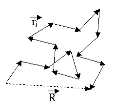
We can derive the MSD of of the FJC Chain model without using a probabilistic perspective as well and this might be a little more intuitive for some people, at least it was for me. Again remember that in the random walk or ideal model we ignore bonding and it is really unphysical in most cases. The end-to-end distance of the Ideal Chain/FJC model can be derived using a different mathematical formalism, sometimes referred to as the Mathematician’s Ideal Chain. We again assume n monomers with a fixed monomer length l and which is represented as a vector in 3D spacewhere this vector refers to monomer i.

So the end to end distance vector is:

$$\vec{r} = \vec{l_1} + \vec{l_2} + \dots + \vec{l_n} = \sum_{i=1}^{n} \vec{l_i} \nonumber$$

On average what will be the value of $\langle \vec{r} \rangle$? Remember that for the ideal polymer chain, each step positive or negative is equally likely, these steps are uncorrelated. So on average the value of $\langle \vec{r} \rangle = 0$.

The better question is what will be $\langle \vec{r}^2 \rangle$ and we can write this as the dot product:

$$\langle \vec{r}_i \cdot \vec{r}_j \rangle = \langle \sum_{i=1}^{n} \vec{l}_i \cdot \sum_{j=1}^{n} \vec{l}_j \rangle \nonumber$$

where i and j refer to monomer i and monomer j. Remember that the dot product is:

$$\vec{l}_i \cdot \vec{l}_j = |l_i||l_j| \cos \theta_{ij} \nonumber$$

We can show the MSD in matrix notation as well:

$$\langle \vec{r}_i \cdot \vec{r}_j \rangle = \begin{bmatrix} \vec{l_1} \cdot \vec{l_1} & \vec{l_1} \cdot \vec{l_2} & \vec{l_1} \cdot \vec{l_3} & \dots & \vec{l_1} \cdot \vec{l_n} \\ \vec{l_2} \cdot \vec{l_1} & \vec{l_2} \cdot \vec{l_2} & \dots & \\ \vdots & & & \ddots & \\ \vec{l_n} \cdot \vec{l_1} & \dots & & \vec{l_n} \cdot \vec{l_n} \end{bmatrix} \nonumber$$

Now let's think about the value of the dot product on the diagonal component. The magnitude will simply be $l^2$ for every component, but now we need to think about the $\cos \theta$ between the two vectors. Well, for the diagonal component, they will always be pointing in the same direction, so the angle will be $0^\circ$ and then $\cos 0^\circ = 1$.

Now for the off-diagonal components. Let's keep it simple and think about the 1D scenario. Well, there the value of $\cos \theta = 1$ or $-1$. But remember we are concerned about the averages, so since both positive and negative steps are equally probable (Markov/Monte Carlo) or uncorrelated, so on average the value of $\cos \theta = 0$.

So the matrix reduces to:

$$\langle \vec{r}_i \cdot \vec{r}_j \rangle = \begin{bmatrix} l^2 & 0 & 0 & \dots & 0 \\ 0 & l^2 & \dots & \\ \vdots & & & \ddots & \\ 0 & \dots & & & l^2 \end{bmatrix} \nonumber$$

Thus the sum of this matrix becomes:

$$\langle r^2 \rangle = n l^2 \nonumber$$

just as we obtained previously with our other probabilistic method!

The Chemist’s Polymer Chain Model

So far we have neglected a lot of detail in describing polymer chains that make the previous models a bit unphysical. We have neglected taking into account restrictions in bond angles to to steric hindrance along the backbone chain a well as any solvent effect and how that may affect the end-to-end distance of the polymer chain.

Here, we will introduce two new effective parameters, C_∞ and α, that can be used to correct for problems in the simple random walk model end-to-end distance based on known bonding constraints and solvent considerations. Note that in a random walk, C_∞ = α = 1. The parameter C_∞ is used to take into account restrictions due to bonding and steric hindrance from the polymer chain, while the parameter α takes into account effects from the solvent. This improved models is referred to as the Chemist’s Polymer Chain in Solution and Melt model. This model is more physically accurate as this model considers bond angle restrictions between adjacent atoms (or monomers) due to chemistry.

This governing equation for the Chemist's model is:

$$\langle r^2 \rangle = nl^2 C_\infty \alpha^2 \nonumber$$

Let's figure out where these new values come from, starting with going back to the matrix that we developed in the FJC model. In the Chemist's Model, we assume that we have a fixed bond angle $\theta$, which makes sense thinking of polyethylene. Now, the dot product of monomer $i$ and $i+1$ will be:

$$\vec{l_{i}} \cdot \vec{l_{i+m}} = l^{2} (-\cos \theta)^m \nonumber$$

where $m$ is an integer denoting the number of monomers away from monomer $i$, and $\theta$ keeps getting multiplied because of the projection of the bond onto the next neighbor. You can see this model schematically here.

Now we can adjust our previous matrix and get:

$$\langle \vec{r}_i \cdot \vec{r}_j \rangle = \begin{bmatrix} l^2 & l^2(-\cos \theta) & l^2(\cos \theta)^2 & \dots & l^2(- \cos \theta)^{n-1} \\ l^2(-\cos \theta) & l^2 & \dots & \\ \vdots & & & \ddots \\ l^2 (- \cos \theta)^{n-1} & \dots & & & l^2 \\ \end{bmatrix} \nonumber$$

And once you sum this matrix, we find that:

$$\langle r^2 \rangle = nl^2 \left( \frac{1 - \cos \theta}{1 + \cos \theta} \right) \nonumber$$

This factor of $\frac{1 - \cos \theta}{1 + \cos \theta}$ is:

$$C_{\infty} = \frac{1 - \cos \theta}{1 + \cos \theta} \nonumber$$

So we now get that:

$$\langle r^2 \rangle = n l^2 C_{\infty} \nonumber$$

where $C_{\infty}$ is the Flory characteristic ratio, which can be thought of as a measure of the stiffness of your monomer unit or how hard it is to rotate. You can look up this ratio for a number of different polymers, and we should know that for C-C bonds, $\theta = 109.5^\circ$. Much more on Flory to come.

Rotational Isomeric States

Now, this is an improvement, but we have missed something very important, and it is related to our discussion of conformers vs. isomers. We have previously briefly mentioned that there are certain molecules with different isomeric states, i.e., the same chemical formula but distinct structures that can't be related via rotation around a bond. A conformer or conformational isomer can be related to different structures via rotations around a single bond, and these different rotational states are called rotational isomeric states (RIS). Additionally, these different states will each have different potential energies, and thus we will find these different RIS states according to the weighted probabilities determined by the rotational potential $V(\phi)$. We can see the different RIS states of a conformer like n-butane here.

Here, there are clearly high-energy states where the bulky methyl groups overlap with either a hydrogen or another methyl group. Then we have our lower energy conformation, as seen denoted by gauche $\pm$, and the lowest energy being the trans conformation. I wanted to illustrate this example because we did not treat this case in our derivation of the Chemist's chain model, so we need to take this into account. Luckily, we can do so using a very similar train of logic as we did above, but instead of simply using a fixed $\cos \theta$, we need to take an ensemble average of the RIS angles based on the number of microstates for each angle, so we will use:

$$\langle \cos \phi \rangle = \frac{\int \cos \phi V(\phi) d \phi}{\int V(\phi) d \phi} \nonumber$$

And we eventually end up with (skipping the full derivation as it is very, very, extremely difficult):

$$\langle r^2 \rangle = nl^2 \left[ \left( \frac{1 - \cos \theta}{1 + \cos \theta} \right) \left( \frac{1 + \langle \cos \phi \rangle}{1 - \langle \cos \phi \rangle} \right) \right] \nonumber$$

And now we have our new and improved Flory Characteristic Ratio $C_{\infty}$, which is:

$$C_{\infty} = \left( \frac{1 - \cos \theta}{1 + \cos \theta} \right) \left( \frac{1 + \langle \cos \phi \rangle}{1 - \langle \cos \phi \rangle} \right) \nonumber$$

This derivation is beyond the scope of this course, but you can look it up in Statistical Mechanics of Chain Molecules if you're interested, which is Flory's text. Again, much more Flory to come. Also, some refer to this addition as the Hindered Rotation model.

Let's take a moment here to appreciate what we have just done. By taking into account bond angles and rotations, we get fairly accurate values of $C_{\infty}$ compared to experimental measurements, and usually, this value varies between 1-20. It's important to note that $C_{\infty}$ must always be at least 1, and this implies that the FJC/ideal chain is the most coiled conformation. This makes sense because by restricting these bond rotations, we are inherently expanding our polymer chain, leading to a more elongated polymer.

However, our work is not finished yet. We have taken into account bond angles and bond rotation, but what else must we consider? Well, does this model make any distinction between polymers that might have a large or bulky side chain? No! For these polymers with large bulky side chains, we should expect that $C_{\infty}$ should increase as the rotations are more difficult due to steric interactions. So the increase is not due to bonding interactions but due to excluded volume effects.

Excluded Volume

In order to capture these intramolecular steric interactions between monomers we have to talk about a somewhat initially obtuse concept of excluded volume. Excluded volume is the concept that monomers have some volume around them that other molecules can’t cross or move into this sphere. This takes care of the FJC ability of the chain to self-cross. These excluded volume interactions usually occur between monomers far apart on the polymer chain (because they must cross and intersect) and as you might imagine again like the bond angles and rotation this excluded volume effect will increase the $\langle r^2 \rangle$ of the polymer chain.

Now this may still be a bit obtuse but you can visualize this excluded volume as a hard, impenetrable sphere that surround a given molecule or monomer. The size of the sphere must reflect the structure of the monomer. So a monomer, like polystyrene with a large bulky phenyl group will have a larger excluded volume than polyethylene with it’s hydrogen groups and no side chain. This excluded volume interaction will also depend on the interactions of the monomer with solvent interactions. If the monomer doesn’t like to interact with the solvent then the polymer will want to coil and collapse to avoid these interactions and thus the excluded volume will decreases and vice versa. Remember that the solvent is the majority component and solute is the minority component.

Effect of Solvent on Polymer Chain MSD

Speaking of solvent effect...as we mentioned in our Polymerization lecture there are times when the polymer is immersed in some type of solvent (i.e. water, alcohol, organic solvent, etc.). This solvent can have serious consequences on the dimension of our polymer chain. In good solvents, i.e. solvents were the polymer likes to interact with the solvent (favorable enthalpic intermolecular interactions), the polymer will extend in order to maximize the number of interactions between monomer and solvent. Conversely, if we are dealing with a bad solvent then the polymer doesn’t want to interact with the solvent and the polymer chain will fold in on itself and coil in order to minimize interactions with the solvent and the end-to-end distance will decrease. In the FJC/Ideal model we are in a very special condition with regards to solvent in that we are in a θ condition and thus in a theta solvent. In this condition you can imagine that upon mixing a polymer chain and a solvent the enthalpy of mixing is 0 just like an ideal solution. Alternatively you can imagine that excluded volume of the polymer chain does not change upon adding a θ solvent.

The parameter that we use to quantify the effect of solvent quality is measured via a factor α. Luckily α is a fairly simple quantity to measure and is simply the ratio of the MSD end-to-end distance of the real chain in solution vs the chain in a θ solvent

$$\alpha^2 = \frac{\langle r^2 \rangle}{\langle r^2 \rangle_{\theta}} \nonumber$$

where $\langle r^2 \rangle_{\theta}$ is the MSD of the chain in a θ solvent. So let’s define some values of α.

What will be the value of α in a good solvent?

Well α > 1 for a good solvent.

What about a bad solvent? α < 1 for a bad solvent What about a θ solvent? α = 1 for a θ solvent

We will be talking much more about enthalpic interactions when we discuss Flory and whether enthalpic interactions are good/favorable and whether they are bad/poor/unfavorable interactions. We will talk about monomer-monomer interactions ($\epsilon_{m-m}$), monomer-solvent interactions ($\epsilon_{m-s}$), and solvent-solvent interactions ($\epsilon_{s-s}$). Remember from the thermodynamic lecture that we always want lower or negative energies, so for a good solvent $\epsilon_{m-s}$ should be the lowest energetic interaction, and for a bad solvent, $\epsilon_{m-s}$ should be larger. Much more on this when we get to Flory.

Physicist’s Ideal Chain

The last model is the Physicist’s Ideal Chain. Here we take a coarse-grained approach and approximate larger chains as freely jointed chains. We then change the values of n and l to N and b to reflect a larger length scale, where b is the Kuhn length. This model holds for a chain in θ condition or in the melt state, where the polymer chain is not in solvent (again we will discuss this more in depth once we get to Flory). Essentially, all the work that we have just done in defining C_∞ is encapsulated in these terms as seen below

$$N = \frac{n}{C_{\infty}} \nonumber$$

$$b = C_{\infty} l \nonumber$$

Radius of Gyration

Now before we move we should consider that polymers are not all simple linear chains. We encounter star, dendrimers, branched, and many other complex architectures and it becomes much more complicated to measure the average mean squared end-to-end distance. For these polymers we will typically calculate the radius of gyration which is

$$r^{2}_{g} = \frac{1}{n} \sum_{i=1}^{n} (\vec{r}_{i} - r_{cm})^2 \nonumber$$

where r_cm is the center of mass of the polymer as seen below

$$\vec{r}_{cm} = \frac{\sum_{j=1}^{n} M_{j}\vec{r}_{j}}{\sum_{j=1}^{n} M_{j}} \nonumber$$

Figure 8. Physicist’s Ideal Chain

but typically we know that the monomer mass M will be the same for all monomers so M_j = M_o and we can re-write the position vector of the center of mass as

$$\vec{r}_{cm} = \frac{1}{n} \sum_{j=1}^{n} M_{j}\vec{r}_{j} \nonumber$$

This is a very useful parameter because you can calculate this if the polymer is branched, crosslinked, or a comb as well. The radius of gyration is simply the mean squared end-to-end distance from the center of mass divided by the number of monomers. This also gives us an idea of the mass density distribution of the polymer as well.

Now you can derive the radius of gyration for all of the polymer chain models that we will discuss in this lecture but one of the most important relationship is relating the radius of gyration to the ideal linear chain model which is

$$\langle r_{g}^{2} \rangle = \frac{\langle r^2 \rangle}{6} \nonumber$$

Real Polymer Chains : Swelling and Excluded Volume

We have just given a fairly hand-wavy description of the solvent quality parameter α but we have failed to capture the behavior of real chains. Specifically, the interactions between monomers and between monomers and solvent molecules.

We will now include these interactions and derive α explicitly using theory developed by Paul Flory a polymer physicist and Nobel Prize winner. We will also see our first instance of our never ending battle between entropy and enthalpy. We will see the different contributions that effect α, learn how to control or modify α, and the effect it has on properties like viscocity or the end-to-end distance of the chain.

Contributions to Polymer Swelling: Entropic Spring and Excluded Volume

So before we jump into the factors that can cause polymer swelling or polymer coiling let’s start from the the initial unperturbed state where α = 1 and move to it’s final swollen state where α > 1. For most polymers we should expect that in reality the polymer end-to-end distance will always be larger than in the θ solvent case as typically the the monomer-monomer interactions should lead to some mutual repulsion (like-like interactions) and increase the end-to-end distance of the polymer chain.

When thinking about how to describe the contributions to polymer swelling we will typically have

(1) Entropic (Elastic) Contribution: Chain wants to compress and coil to maximize number of configurations/microstates

(2) Enthalpic Contribution: Monomer-monomer interactions (excluded volume) increases chain size, maximize enthalpy

Let’s think about these two contributions starting with the entropic contribution which is sometimes referred to as the entropic spring or entropic restoring force. When the polymer chain is extended via swelling or if you take it to the extreme and we pull and stretch a polymer chain we know that the end-to-end distance distribution of polymer chains follows a Gaussian distribution. By pulling on the polymer chain or swelling a polymer chain we are biasing the distribution and the polymer will adopt much less probable larger end-to-end distances. Doing this decreases the number of microstates and thus decreases the entropy of the system. This is not energetically favorable we want to always increase the entropy of the system. So this induces an entropic restoring force to the undeformed state. You can also call this an entropic spring because the functional form of his entropic restoring force will be very similar to Hooke’s law. So when we swell or pull on a polymer we pay a cost in entropy or pay an entropy energy penalty.

So now what about the enthalpy contribution. When we have a polymer in a solvent the effective interactions between monomers is dependent on the interaction between monomers and the monomers with the solvent. As we have mentioned previously in a good solvent the monomer-monomer interaction is less favorable (higher energy) than the monomer-solvent interactions and vice versa for the poor solvent. In a theta solvent the monomer-solvent interaction counter acts the monomer-monomer interaction so that there is no net interaction, i.e. enthalpy of 0, ideal solution.

So with these two contributions we will have the total free energy as being composed of two contributions which sum

$$G = G_{entropic} + G_{enthalpic} \nonumber$$

where G is the system free energy of the polymer and solvent, G_entropic is the entropic spring contribution and G_enthalpic is the enthalpic contribution. Let’s derive these two contributions to free energy.

Entropic Spring

Let’s start with the entropic spring contribution. We can remember that the probability distribution of an ideal chain is

$$P(r, n) = (\frac{1}{2\pi nl^2})^\frac{3}{2}\exp(-\frac{3r^2}{2nl^2}) \nonumber$$

We want to write an expression for the free energy contribution of the entropic spring, i.e. how the free energy will change as a function of the end-to-end distance of our polymer chain, r. Well we know from our thermodynamics and statistical mechanics lecture that we can relate the number of possible configurations Ω to the entropy

$$S = k \ln \Omega \nonumber$$

When we change the initial end-to-end distance of our initial ideal chain with an endto-end distance of r₀ and a number of monomers n the entropy can be re-written as

$$S (n,r) = k \ln \Omega (n,r) \nonumber$$

where you can see that both the entropy and number of possible configuration will change as a function of the number of monomers and end-to-end distance but typically in the problems that we will work on the number of monomers will be fixed, n, but the end-to-end distance will change.

Now we can write the probability that a polymer assumes a given microstate or configuration for a given number of monomers and end-to-end distance is just as we have described before in our supplementary lecture

$$P(n, r) = \frac{\Omega(n, r)}{\int \Omega(n,r) dr} \nonumber$$

Again quick note that we are working on the assumption that all configurations are equally probable i.e. ideal chain. Thus the probability is just the number of configurations with that particular microstate divided by the total number of configurations. So now we can do some math

$$S(n, r) = k \ln \Omega(n, r) \nonumber$$
$$S(n, r) = k \ln \left[ P(n, r) \int \Omega(n, r) \, dr \right] \nonumber$$
$$S(n, r) = k \ln P(n, r) + k \ln \left[ \int \Omega(n, r) \, dr \right] \nonumber$$
$$S(n, r) = -\frac{3}{2}k\frac{r^2}{n l^2} + \frac{3}{2}k \ln \bigg(\frac{3}{2\pi n l^2}\bigg) + k \ln \left[ \int \Omega(n, r) \, dr \right] \nonumber$$
$$S(n, r) = -\frac{3}{2}k\frac{r^2}{r_0^2} + S(n) \nonumber$$

We have our entropy expression which varies as a function of the ratio between the actual end-to-end distance of the chain r vs the unperturbed or ideal chain distance r₀ which should be familiar $\frac{ r^2}{ r_0^2} = \alpha ^2$. Now this last term is not a function of r and this will become important in just a bit because we always want to find the state of the system at equilibrium which will involve taking the derivative of the free energy with respect to r so this will eventually disappear. Now we can write

$$G_{entropic} (n,r) = H (n,r) - TS(n,r) = \frac{3}{2}kT\frac{r^2}{r_0^2} + S(n) \nonumber$$

where remember we set H to 0 as we are working on the ideal chain assumption. Now you might be concerned about this ratio of distances and at this point we have to state this expression is valid only in tension, i.e. r > r₀. I won’t go into the full derivation but we can modify this expression slightly to include compression and we obtain a more useful equation

$$G(r)_{entropic} = \frac{3kT}{2} \left ( \frac{r^2}{nl^2} + \frac{nl^2}{r^2} \right ) \nonumber$$

Here we see that in tension the first term is large and the second term goes to 0 and vice versa for compression. This make sense as any perturbation from ideal chain conditions will reduce the number of possible microstates and thus decrease entropy!

We can derive a similar expression using a statistical mechanics approach by remembering that

$$P(r) \approx \exp \left ( -\frac{G(r)}{k_b T} \right ) \nonumber$$

Additionally we can also simply our expression for the probability of an ideal chain as follows ignoring the pre-factors. Quick note in this class we will discuss over and over again that scaling behavior is critical when talking about polymer. Prefactors or constants are not critical but scaling behavior is much more important.

$$P(r) \approx \exp \left ( -\frac{3r^2}{2nl^2} \right ) = \exp \left (-\frac{3r^2}{2r_0^2} \right ) \nonumber$$

Note that we have defined $r_{0}^{2} = nl^2$ from the FJC/Ideal chain model. After doing some math we are left with the following expression which is

$$G_{entropic} (n,r) = H (n,r) - TS(n,r) = \frac{3}{2}kT\frac{r^2}{r_0^2} \nonumber$$

where we are missing our additive factor S(n) because of the assumptions and getting rid of our pre-factors. Again we can also relate this expression for the entropic or elastic free energy contribution directly to the solvent quality parameter.

Enthalpic/Excluded Volume Interactions:

Now, we need to write an expression which considers the monomer-monomer interactions. Well to start we can remember back to Materials to our LJ potential and treat the monomers as hard spheres and look at the potential between the spheres as shown below

$$V_{LJ} = 4\epsilon \bigg[\bigg(\frac{\sigma}{r} \bigg)^{12} - \bigg(\frac{\sigma}{r} \bigg)^{6}\bigg] = \epsilon \bigg[\bigg(\frac{r_{o}}{r} \bigg)^{12} - 2\bigg(\frac{r_{m}}{r} \bigg)^{6}\bigg] \nonumber$$

where is the depth of the potential well, σ is the distance at which the inter-particle potential is zero, r is the distance between particles, and r_m is the distance where the potential is minimized. This is a very specific potential and this expression will change for different interactions but this is a starting point for what we will discuss.

At short distances the potential will increase (energetically unfavorable) due to overlap of electron clouds. At larger distance the potential will be slightly negative but will approach 0 as the monomers are too far away to interact. At some equilibrium distance there will either be a well or a hill in the curve and this will depend on the solvent quality. Lower energy will always denote a more favorable interaction so in poor solvents where we know that the monomer-monomer interaction is more favorable we will see a well and most likely a deep well. For good solvent this well will be much more shallow or even become positive and create an energy hill. The depth of the well or hill is given by .

Again we can also find the probability of finding two monomers separated by a given distance r is

$$P(r) = \exp \bigg(-\frac{U(r)}{k_b T}\bigg) \nonumber$$

which you can see here and we can see that probability matches our discussion above. Note that at very large values of r the energy goes to zero and thus the exponential of 0 is 1.

Now in order to find the excluded volume we have to utilize the Mayer f-function, a function that you will work with more often if you take a thermodynamic course which is

$$f(r) = \exp \bigg(-\frac{U(r)}{k_b T}\bigg) - 1 \nonumber$$

All this function effectively does is subtract the probability at large r values. What this function effectively does is describe the relative probability of finding two monomers close to one another versus no interaction at all. The excluded volume is then giving by the integral of this curve

$$v = -\int f(r) dr \nonumber$$

which is also shown schematically here

What this graph shows is that the excluded volume is related to the net probability of finding two monomers close to each other across all space, thus accounting for net interactions between two monomers. The excluded volume is the effective volume occupied by a monomer including interactions with solvent and other monomers as well. We will have v < 0 for net attraction (poor solvent), v = 0 for no interaction (θ solvent), and v > 0 for net repulsion (good solvent).

Let’s take a physical look at what this equation is telling us. Let’s say think about what will happen if the potential has an energy hill or only a repulsive component, no attraction like in the case for a very good solvent. Well then the excluded volume will only be positive and very large which leads to swelling as we might expect. As the attraction between monomers increase the excluded volume will still be positive but with a smaller magnitude and less swelling. At some point the attractive part of the potential will be the same magnitude as the repulsive leading to an excluded volume of 0 which is θ conditions. If the attraction increases further then the excluded volume will become negative the polymer will coil and collapse on itself.

Now that we have defined excluded volume as an interaction between monomers we can derive an expression for the free energy between all the monomers in the chain. Let’s consider a a single monomer in a polymer chain with an excluded volume v and n other monomers in the polymer chain. Now remember what makes polymers and soft matter unique is that the polymer chains interaction are on the order of kT and this produces fluctuations of the polymer chain. So let’s consider a scenario where one of the monomers collides or attempts to occupy the excluded volume of another monomer. The interaction energy between these monomers increases approximately by an amount of kT. We can then approximate the total interaction based on the number of these collisions.

So let’s keep is somewhat simple and say the probability of these interactions will clearly depend one the size of the excluded volume v and the number of monomers n. We will also have to divide by the volume of the chain which we will approximate as V ≈ r³, as the larger the volume of the chain/end-to-end distance the less likely monomers will collide. So this will give us the interaction for a single monomer but we have n monomers in our chain so we have to multiple again by n and divide by 2 to avoid overcounting.

So we can write the free energy density for the enthalpic contribution as

$$\frac{G_{enthalpic}(r)}{V} \approx \frac{kTv}{2}\frac{n^2}{r^6} \nonumber$$

Additionally we can see that the concentration of polymer c as seen below

$$c = \frac{n}{r^3} \nonumber$$

which allows us to write the expression below

$$\frac{G_{enthalpic}(r)}{V} \approx \frac{kTv}{2}c^2 \nonumber$$

Note you can generalize this expression to include many body interactions

$$\frac{G_{enthalpic}}{V} \approx kT \left ( \frac{vc^2}{2} + \frac{wc^3}{6} + ... \right ) \nonumber$$

We can then simply multiply by volume to get our total free energy

$$G_{enthalpic} \approx kT\frac{vc^2r^3}{2} \nonumber$$

Flory Full Free Energy:

Finally we can now combine our two terms to obtain the full Flory Free Energy

$$G = G_{entropic} + G_{enthalpic} = kT \left ( \frac{vc^2r^3}{2} + \frac{wc^3r^3}{6} + ... \right ) + \frac{3kT}{2} \left ( \frac{r^2}{nl^2} + \frac{nl^2}{r^2} \right ) \nonumber$$

We can also re-write this a bit more simply ignoring the prefactors that are on the order of 1 and we can ignore interaction terms beyond 3 body interactions

$$\frac{G}{kT} = vc^2r^3 + wc^3r^3 + \frac{r^2}{nl^2} + \frac{nl^2}{r^2} \nonumber$$

Now we can use our relationship for concentration of polymers and substitute in

$$\frac{G}{kT} = \frac{vn^2}{r^3} + \frac{wn^3}{r^6} + \frac{r^2}{nl^2} + \frac{nl^2}{r^2} \nonumber$$

To obtain free energy we have to take the derivative and set this equal to zero

$$\frac{\partial G/kT}{\partial r} = - \frac{3 v n^2}{r^4} - \frac{6 w n^3}{r^7} + \frac{2r}{n l^2} - \frac{2 n l^2}{r^3} \nonumber$$

$$\frac{\partial G/kT}{\partial r} = - 3 v n^2 - \frac{6 w n^3}{r^3} + \frac{2r^5}{n l^2} - 2 n l^2 r \nonumber$$

Again ignoring prefactors on the order of 1 and dividing by (nl²)^3/2

$$\frac{\partial G/kT}{\partial r} = - \frac{ vn^2}{(nl^2)^{3/2}} - \frac{w}{l^6} \left ( \frac{nl^2}{r^2} \right )^{3/2} + \left ( \frac{r^2}{nl^2} \right )^{5/2} - \left ( \frac{r^2}{nl^2} \right )^{1/2} \nonumber$$

substituting in for α from the Chemists chain model i.e. $\alpha = \bigg ( \frac{r^2}{nl^2} \bigg )^{1/2}$

$$\frac{\partial G/kT}{\partial r} = - \frac{ vn^{1/2}}{l^3} - \frac{w}{l^6}\alpha^{-3} + \alpha^5 - \alpha = 0 \nonumber$$

With this expression in hand we can now explicitly determine the scaling behavior of the end-to-end distance of polymer chains in different solvents.

Scaling Behavior in Solvents:

Good Solvents:

Let’s first consider the Full Free energy expression for a good solvent where we know that v >> 0 and α >> 0. In doing so we can re arrange our expression

$$\alpha^5 - \alpha = \frac{ vn^{1/2}}{l^3} + \frac{w}{l^6}\alpha^{-3} \nonumber$$

We can see in this expression that the α⁻³ term will be essentially 0 and that α⁵ will be much greater than the α term so the expression reduces to

$$\alpha^5 = \frac{ vn^{1/2}}{l^3} \nonumber$$

We can then again use our Chemist’s Chain model definition of α and obtain that

$$\langle r^2 \rangle ^\frac{1}{2} \approx l n^{3/5} \nonumber$$

This is our essential finding! We quantitatively prove what we have been discussing for several weeks that the end-to-end distance will scale differently n^3/5 vs the ideal scenario n^1/2 and that the polymer will expand and swell. This difference of n^1/10 may seem small but remember we have n values up to 100,000.

Now we made a lot of assumptions here but when you run computer simulations of self avoiding random walks (SARW) where lattice sites can only be occupied by one monomer the scaling exponent is 0.588 so Flory was pretty close, he didn’t get a Nobel for no reason.

Poor Solvent

We can do the same analysis for a poor solvent knowing that v < 0 and α << 1. The expression now reduces to

$$\frac{ vn^{1/2}}{l^3} = - \frac{w}{l^6}\alpha^{-3} \nonumber$$

and plugging in for again for α

$$\alpha^3 = \frac{w}{l^6} \frac{l^3}{vn^{1/2}} \nonumber$$

$$\alpha = \left( \frac{w}{vn^{1/2}l^3} \right)^{1/3} \nonumber$$

$$\frac{r}{n^{1/2}l} = \left( \frac{w}{vn^{1/2}l^3} \right)^{1/3} \nonumber$$

$$\langle r^2 \rangle^{1/2} \approx \left( \frac{w}{v} \right)^{1/3} n^{1/3} \nonumber$$

Here again we care about the scaling behavior so that pre-factor doesn’t matter to use and we see that $\langle r^2 \rangle ^\frac{1}{2} \approx n^{1/3}$ so this scaling is smaller than the ideal polymer chain so this polymer will be more coiled and collapsed and this all matches our intuition.

Theta Solvent

In a theta solvent we know that v = 0 and the three body parameter w = 0. This leads to an α = 1 and we obtain our typical scaling for a theta solvent.

This concludes our analysis where we had two competing factors that we had to deal with to reach our thermodynamic state of equilibrium: a compressive elastic contribution that arises from an entropic spring restoring force and an expansive excluded volume effect from enthalpic interactions between polymer segments. Don’t worry though we will do a similar analysis many more times in this class.

So to quickly summarize

(1) Mathematician’s Ideal Random Walk/Ideal Chain Model $\langle r^2 \rangle =nl^2$

• Assumes freely jointed chain, no bond angles, polymer can cross itself, no RIS states, steric interactions, or solvent/excluded volume interactions. Captures behavior of θ solvent and melt state fairly well.

(2) Chemist’s Chain Model In Solution and Melt $\langle r^2 \rangle = n l^2 C_\infty \alpha^2$

• θ Solvent or Melt $\langle r^2 \rangle \approx nl^2$

• Good Solvent $\langle r^2 \rangle \approx n^\frac{6}{5}$

• Poor Solvent $\langle r^2 \rangle \approx n^{2/3}$

• Takes into account preferred bond angles, steric interactions, RIS states, solvent, and excluded volume interactions.

(3) Physicist’s Universal Chain $\langle r^2 \rangle = N b^2$

• Simplifies previous the Chemist’s chain by incorporating the Flory parameter into the Kuhn length b, accurate for θ solvent and melt.