
Density of States
- Page ID
- 312
\( \newcommand{\vecs}[1]{\overset { \scriptstyle \rightharpoonup} {\mathbf{#1}} } \)
\( \newcommand{\vecd}[1]{\overset{-\!-\!\rightharpoonup}{\vphantom{a}\smash {#1}}} \)
\( \newcommand{\dsum}{\displaystyle\sum\limits} \)
\( \newcommand{\dint}{\displaystyle\int\limits} \)
\( \newcommand{\dlim}{\displaystyle\lim\limits} \)
\( \newcommand{\id}{\mathrm{id}}\) \( \newcommand{\Span}{\mathrm{span}}\)
( \newcommand{\kernel}{\mathrm{null}\,}\) \( \newcommand{\range}{\mathrm{range}\,}\)
\( \newcommand{\RealPart}{\mathrm{Re}}\) \( \newcommand{\ImaginaryPart}{\mathrm{Im}}\)
\( \newcommand{\Argument}{\mathrm{Arg}}\) \( \newcommand{\norm}[1]{\| #1 \|}\)
\( \newcommand{\inner}[2]{\langle #1, #2 \rangle}\)
\( \newcommand{\Span}{\mathrm{span}}\)
\( \newcommand{\id}{\mathrm{id}}\)
\( \newcommand{\Span}{\mathrm{span}}\)
\( \newcommand{\kernel}{\mathrm{null}\,}\)
\( \newcommand{\range}{\mathrm{range}\,}\)
\( \newcommand{\RealPart}{\mathrm{Re}}\)
\( \newcommand{\ImaginaryPart}{\mathrm{Im}}\)
\( \newcommand{\Argument}{\mathrm{Arg}}\)
\( \newcommand{\norm}[1]{\| #1 \|}\)
\( \newcommand{\inner}[2]{\langle #1, #2 \rangle}\)
\( \newcommand{\Span}{\mathrm{span}}\) \( \newcommand{\AA}{\unicode[.8,0]{x212B}}\)
\( \newcommand{\vectorA}[1]{\vec{#1}} % arrow\)
\( \newcommand{\vectorAt}[1]{\vec{\text{#1}}} % arrow\)
\( \newcommand{\vectorB}[1]{\overset { \scriptstyle \rightharpoonup} {\mathbf{#1}} } \)
\( \newcommand{\vectorC}[1]{\textbf{#1}} \)
\( \newcommand{\vectorD}[1]{\overrightarrow{#1}} \)
\( \newcommand{\vectorDt}[1]{\overrightarrow{\text{#1}}} \)
\( \newcommand{\vectE}[1]{\overset{-\!-\!\rightharpoonup}{\vphantom{a}\smash{\mathbf {#1}}}} \)
\( \newcommand{\vecs}[1]{\overset { \scriptstyle \rightharpoonup} {\mathbf{#1}} } \)
\(\newcommand{\longvect}{\overrightarrow}\)
\( \newcommand{\vecd}[1]{\overset{-\!-\!\rightharpoonup}{\vphantom{a}\smash {#1}}} \)
\(\newcommand{\avec}{\mathbf a}\) \(\newcommand{\bvec}{\mathbf b}\) \(\newcommand{\cvec}{\mathbf c}\) \(\newcommand{\dvec}{\mathbf d}\) \(\newcommand{\dtil}{\widetilde{\mathbf d}}\) \(\newcommand{\evec}{\mathbf e}\) \(\newcommand{\fvec}{\mathbf f}\) \(\newcommand{\nvec}{\mathbf n}\) \(\newcommand{\pvec}{\mathbf p}\) \(\newcommand{\qvec}{\mathbf q}\) \(\newcommand{\svec}{\mathbf s}\) \(\newcommand{\tvec}{\mathbf t}\) \(\newcommand{\uvec}{\mathbf u}\) \(\newcommand{\vvec}{\mathbf v}\) \(\newcommand{\wvec}{\mathbf w}\) \(\newcommand{\xvec}{\mathbf x}\) \(\newcommand{\yvec}{\mathbf y}\) \(\newcommand{\zvec}{\mathbf z}\) \(\newcommand{\rvec}{\mathbf r}\) \(\newcommand{\mvec}{\mathbf m}\) \(\newcommand{\zerovec}{\mathbf 0}\) \(\newcommand{\onevec}{\mathbf 1}\) \(\newcommand{\real}{\mathbb R}\) \(\newcommand{\twovec}[2]{\left[\begin{array}{r}#1 \\ #2 \end{array}\right]}\) \(\newcommand{\ctwovec}[2]{\left[\begin{array}{c}#1 \\ #2 \end{array}\right]}\) \(\newcommand{\threevec}[3]{\left[\begin{array}{r}#1 \\ #2 \\ #3 \end{array}\right]}\) \(\newcommand{\cthreevec}[3]{\left[\begin{array}{c}#1 \\ #2 \\ #3 \end{array}\right]}\) \(\newcommand{\fourvec}[4]{\left[\begin{array}{r}#1 \\ #2 \\ #3 \\ #4 \end{array}\right]}\) \(\newcommand{\cfourvec}[4]{\left[\begin{array}{c}#1 \\ #2 \\ #3 \\ #4 \end{array}\right]}\) \(\newcommand{\fivevec}[5]{\left[\begin{array}{r}#1 \\ #2 \\ #3 \\ #4 \\ #5 \\ \end{array}\right]}\) \(\newcommand{\cfivevec}[5]{\left[\begin{array}{c}#1 \\ #2 \\ #3 \\ #4 \\ #5 \\ \end{array}\right]}\) \(\newcommand{\mattwo}[4]{\left[\begin{array}{rr}#1 \amp #2 \\ #3 \amp #4 \\ \end{array}\right]}\) \(\newcommand{\laspan}[1]{\text{Span}\{#1\}}\) \(\newcommand{\bcal}{\cal B}\) \(\newcommand{\ccal}{\cal C}\) \(\newcommand{\scal}{\cal S}\) \(\newcommand{\wcal}{\cal W}\) \(\newcommand{\ecal}{\cal E}\) \(\newcommand{\coords}[2]{\left\{#1\right\}_{#2}}\) \(\newcommand{\gray}[1]{\color{gray}{#1}}\) \(\newcommand{\lgray}[1]{\color{lightgray}{#1}}\) \(\newcommand{\rank}{\operatorname{rank}}\) \(\newcommand{\row}{\text{Row}}\) \(\newcommand{\col}{\text{Col}}\) \(\renewcommand{\row}{\text{Row}}\) \(\newcommand{\nul}{\text{Nul}}\) \(\newcommand{\var}{\text{Var}}\) \(\newcommand{\corr}{\text{corr}}\) \(\newcommand{\len}[1]{\left|#1\right|}\) \(\newcommand{\bbar}{\overline{\bvec}}\) \(\newcommand{\bhat}{\widehat{\bvec}}\) \(\newcommand{\bperp}{\bvec^\perp}\) \(\newcommand{\xhat}{\widehat{\xvec}}\) \(\newcommand{\vhat}{\widehat{\vvec}}\) \(\newcommand{\uhat}{\widehat{\uvec}}\) \(\newcommand{\what}{\widehat{\wvec}}\) \(\newcommand{\Sighat}{\widehat{\Sigma}}\) \(\newcommand{\lt}{<}\) \(\newcommand{\gt}{>}\) \(\newcommand{\amp}{&}\) \(\definecolor{fillinmathshade}{gray}{0.9}\)1.1 Introduction
The density of states (DOS) is essentially the number of different states at a particular energy level that electrons are allowed to occupy, i.e. the number of electron states per unit volume per unit energy. Bulk properties such as specific heat, paramagnetic susceptibility, and other transport phenomena of conductive solids depend on this function. DOS calculations allow one to determine the general distribution of states as a function of energy and can also determine the spacing between energy bands in semi-conductors\(^{[1]}\).
1.2 Density of States for Waves
Before we get involved in the derivation of the DOS of electrons in a material, it may be easier to first consider just an elastic wave propagating through a solid. Elastic waves are in reference to the lattice vibrations of a solid comprised of discrete atoms. Though, when the wavelength is very long, the atomic nature of the solid can be ignored and we can treat the material as a continuous medium\(^{[2]}\).
We begin with the 1-D wave equation: \( \dfrac{\partial^2u}{\partial x^2} - \dfrac{\rho}{Y} \dfrac{\partial u}{\partial t^2} = 0\)
With which we then have a solution for a propagating plane wave:
\[u = A e^{i(qx-\omega t)} \]
\(q\)= wave number: \(q=\dfrac{2\pi}{\lambda}\), \(A\)= amplitude, \(\omega\)= the frequency, \(v_s\)= the velocity of sound
Dispersion Relations:
\[ \omega = \nu_s q\nonumber\]
In equation(1), the temporal factor, \(-\omega t\) can be omitted because it is not relevant to the derivation of the DOS\(^{[2]}\). So now we will use the solution:
\[ u =Ae^{i(qx)}\]
To begin, we must apply some type of boundary conditions to the system. The easiest way to do this is to consider a periodic boundary condition. With a periodic boundary condition we can imagine our system having two ends, one being the origin, 0, and the other, \(L\). We now say that the origin end is constrained in a way that it is always at the same state of oscillation as end L\(^{[2]}\).
This boundary condition is represented as: \( u(x=0)=u(x=L)\)
Now we apply the boundary condition to equation (2) to get: \( e^{iqL} =1\)
Now, using Euler’s identity; \( e^{ix}= \cos(x) + i\sin(x)\) we can see that there are certain values of \(qL\) which satisfy the above equation. Those values are \(n2\pi\) for any integer, \(n\). Leaving the relation: \( q =n\dfrac{2\pi}{L}\)
If you choose integer values for \(n\) and plot them along an axis \(q\) you get a 1-D line of points, known as modes, with a spacing of \({2\pi}/{L}\) between each mode.
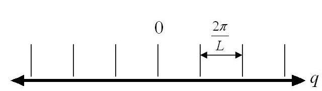
As \(L \rightarrow \infty , q \rightarrow \text{continuum}\).
We now have that the number of modes in an interval \(dq\) in \(q\)-space equals:
\[ \dfrac{dq}{\dfrac{2\pi}{L}} = \dfrac{L}{2\pi} dq\nonumber\]
Using the dispersion relation we can find the number of modes within a frequency range \(d\omega\) that lies within\((\omega,\omega+d\omega)\). This number of modes in that range is represented by \(g(\omega)d\omega\), where \(g\omega\) is defined as the density of states.So now we see that \(g(\omega) d\omega =\dfrac{L}{2\pi} dq\) which we turn into: \(g(\omega)={(\frac{L}{2\pi})}/{(\frac{d\omega}{dq})}\)
We do so in order to use the relation: \(\dfrac{d\omega}{dq}=\nu_s\)
and obtain: \(g(\omega) = \left(\dfrac{L}{2\pi}\right)\dfrac{1}{\nu_s} \Rightarrow (g(\omega)=2 \left(\dfrac{L}{2\pi} \dfrac{1}{\nu_s} \right)\)
we multiply by a factor of two be cause there are modes in positive and negative \(q\)-space, and we get the density of states for a phonon in 1-D:
\[ g(\omega) = \dfrac{L}{\pi} \dfrac{1}{\nu_s}\nonumber\]
2-D
We can now derive the density of states for two dimensions. Equation(2) becomes: \(u = A^{i(q_x x + q_y y)}\)
now apply the same boundary conditions as in the 1-D case:
\[ e^{i[q_xL + q_yL]} = 1 \Rightarrow (q_x,q)_y) = \left( n\dfrac{2\pi}{L}, m\dfrac{2\pi}{L} \right)\nonumber\]
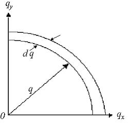
We now consider an area for each point in \(q\)-space =\({(2\pi/L)}^2\) and find the number of modes that lie within a flat ring with thickness \(dq\), a radius \(q\) and area: \(\pi q^2\)
Number of modes inside interval: \(\frac{d}{dq}{(\frac{L}{2\pi})}^2\pi q^2 \Rightarrow {(\frac{L}{2\pi})}^2 2\pi qdq\)
Now account for transverse and longitudinal modes (multiply by a factor of 2) and set equal to \(g(\omega)d\omega\) We get
\[g(\omega)d\omega=2{(\frac{L}{2\pi})}^2 2\pi qdq\nonumber\]
and apply dispersion relation to get \(2{(\frac{L}{2\pi})}^2 2\pi(\frac{\omega}{\nu_s})\frac{d\omega}{\nu_s}\)
which simplifies to the 2-D result:
3-D
We can now derive the density of states for three dimensions. Equation(2) becomes: \(u = A^{i(q_x x + q_y y+q_z z)}\)
now apply the same boundary conditions as in the 1-D case to get:
\[e^{i[q_x x + q_y y+q_z z]}=1 \Rightarrow (q_x , q_y , q_z)=(n\frac{2\pi}{L},m\frac{2\pi}{L}l\frac{2\pi}{L})\nonumber\]
We now consider a volume for each point in \(q\)-space =\({(2\pi/L)}^3\) and find the number of modes that lie within a spherical shell, thickness \(dq\), with a radius \(q\) and volume: \(4/3\pi q ^3\)
Number of modes inside shell:
\[\frac{d}{dq}{(\frac{L}{2\pi})}^3\frac{4}{3}\pi q^3 \Rightarrow {(\frac{L}{2\pi})}^3 4\pi q^2 dq\nonumber\]
Assuming a common velocity for transverse and longitudinal waves we can account for one longitudinal and two transverse modes for each value of \(q\) (multiply by a factor of 3) and set equal to \(g(\omega)d\omega\):
\[g(\omega)d\omega=3{(\frac{L}{2\pi})}^3 4\pi q^2 dq\nonumber\]
Apply dispersion relation and let \(L^3 = V\) to get \[3\frac{V}{{2\pi}^3}4\pi{{(\frac{\omega}{nu_s})}^2}\frac{d\omega}{nu_s}\nonumber\]
and simplify for the 3-D result:
Density of States for Electrons
Now that we have seen the distribution of modes for waves in a continuous medium, we move to electrons. The calculation of some electronic processes like absorption, emission, and the general distribution of electrons in a material require us to know the number of available states per unit volume per unit energy. The density of states is once again represented by a function \(g(E)\) which this time is a function of energy and has the relation \(g(E)dE\) = the number of states per unit volume in the energy range: \((E, E+dE)\).
We begin by observing our system as a free electron gas confined to points \(k\) contained within the surface. We do this so that the electrons in our system are free to travel around the crystal without being influenced by the potential of atomic nuclei\(^{[3]}\). Using the Schrödinger wave equation we can determine that the solution of electrons confined in a box with rigid walls, i.e. the Particle in a box problem, gives rise to standing waves for which the allowed values of \(k\) are expressible in terms of three nonzero integers, \(n_x,n_y,n_z\)\(^{[1]}\).
Taking a step back, we look at the free electron, which has a momentum,\(p\) and velocity,\(v\), related by \(p=mv\). Since the energy of a free electron is entirely kinetic we can disregard the potential energy term and state that the energy, \(E = \dfrac{1}{2} mv^2\)
Using De-Broglie’s particle-wave duality theory we can assume that the electron has wave-like properties and assign the electron a wave number \(k\): \(k=\frac{p}{\hbar}\)
\(\hbar\) is the reduced Planck’s constant: \(\hbar=\dfrac{h}{2\pi}\)
Now we substitute terms:
\[k=\frac{p}{\hbar} \Rightarrow k=\frac{mv}{\hbar} \Rightarrow v=\frac{\hbar k}{m}\nonumber\]
Substitute \(v\) term into the equation for energy:
\[E=\frac{1}{2}m{(\frac{\hbar k}{m})}^2\nonumber\]
We are now left with the dispersion relation for electron energy: \(E =\dfrac{\hbar^2 k^2}{2 m^{\ast}}\)
where \(m ^{\ast}\) is the effective mass of an electron.
As for the case of a phonon which we discussed earlier, the equation for allowed values of \(k\) is found by solving the Schrödinger wave equation with the same boundary conditions that we used earlier.
We are left with the solution: \(u=Ae^{i(k_xx+k_yy+k_zz)}\)
and after applying the same boundary conditions used earlier:
\[e^{i[k_xx+k_yy+k_zz]}=1 \Rightarrow (k_x,k_y,k_z)=(n_x \frac{2\pi}{L}, n_y \frac{2\pi}{L}), n_z \frac{2\pi}{L})\nonumber\]
We can consider each position in \(k\)-space being filled with a cubic unit cell volume of:
\(V={(2\pi/ L)}^3\) making the number of allowed \(k\) values per unit volume of \(k\)-space:\(1/(2\pi)^3\)
We can picture the allowed values from \(E =\dfrac{\hbar^2 k^2}{2 m^{\ast}}\) as a sphere near the origin with a radius \(k\) and thickness \(dk\). The allowed states are now found within the volume contained between \(k\) and \(k+dk\), see Figure \(\PageIndex{1}\).
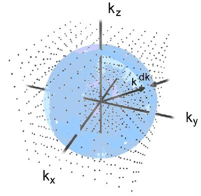
Figure \(\PageIndex{1}\)\(^{[1]}\). Spherical shell showing values of \(k\) as points. The points contained within the shell \(k\) and \(k+dk\) are the allowed values.
The volume of the shell with radius \(k\) and thickness \(dk\) can be calculated by simply multiplying the surface area of the sphere, \(4\pi k^2\), by the thickness, \(dk\):
\[V_{shell}=4\pi k^2 dk\nonumber\]
Now we can form an expression for the number of states in the shell by combining the number of allowed \(k\) states per unit volume of \(k\)-space with the volume of the spherical shell seen in Figure \(\PageIndex{1}\).
Number of states: \(\frac{1}{{(2\pi)}^3}4\pi k^2 dk\)
Substitute in the dispersion relation for electron energy:
\(E =\dfrac{\hbar^2 k^2}{2 m^{\ast}} \Rightarrow k=\sqrt{\dfrac{2 m^{\ast}E}{\hbar^2}}\)
which leads to \(\dfrac{dk}{dE}={(\dfrac{2 m^{\ast}E}{\hbar^2})}^{-1/2}\dfrac{m^{\ast}}{\hbar^2}\) now substitute the expressions obtained for \(dk\) and \(k^2\) in terms of \(E\) back into the expression for the number of states:
\(\Rightarrow\frac{1}
Callstack:
    at (Bookshelves/Materials_Science/Supplemental_Modules_(Materials_Science)/Electronic_Properties/Density_of_States), /content/body/div[3]/p[27]/span, line 1, column 3
\(\Rightarrow\frac{1}{{(2\pi)}^3}4\pi{(\dfrac{2 m^{\ast}}{\hbar^2})}^2{(\dfrac{2 m^{\ast}}{\hbar^2})}^{-1/2})E(E^{-1/2})dE\)
\(\Rightarrow\frac{1}{{(2\pi)}^3}4\pi{(\dfrac{2 m^{\ast}E}{\hbar^2})}^{3/2})E^{1/2}dE\)
We have now represented the electrons in a 3 dimensional \(k\)-space, similar to our representation of the elastic waves in \(q\)-space, except this time the shell in \(k\)-space has its surfaces defined by the energy contours \(E(k)=E\) and \(E(k)=E+dE\), thus the number of allowed \(k\) values within this shell gives the number of available states and when divided by the shell thickness, \(dE\), we obtain the function \(g(E)\)\(^{[2]}\).
\[g(E)=\frac{1}{{4\pi}^2}{(\dfrac{2 m^{\ast}E}{\hbar^2})}^{3/2})E^{1/2}\nonumber\]
we must now account for the fact that any \(k\) state can contain two electrons, spin-up and spin-down, so we multiply by a factor of two to get:
\[g(E)=\frac{1}{{2\pi}^2}{(\dfrac{2 m^{\ast}E}{\hbar^2})}^{3/2})E^{1/2}\nonumber\]
The above expression for the DOS is valid only for the region in \(k\)-space where the dispersion relation \(E =\dfrac{\hbar^2 k^2}{2 m^{\ast}}\) applies. As the energy increases the contours described by \(E(k)\) become non-spherical, and when the energies are large enough the shell will intersect the boundaries of the first Brillouin zone, causing the shell volume to decrease which leads to a decrease in the number of states. If the volume continues to decrease, \(g(E)\) goes to zero and the shell no longer lies within the zone. The energy at which \(g(E)\) becomes zero is the location of the top of the valance band and the range from where \(g(E)\) remains zero is the band gap\(^{[2]}\).
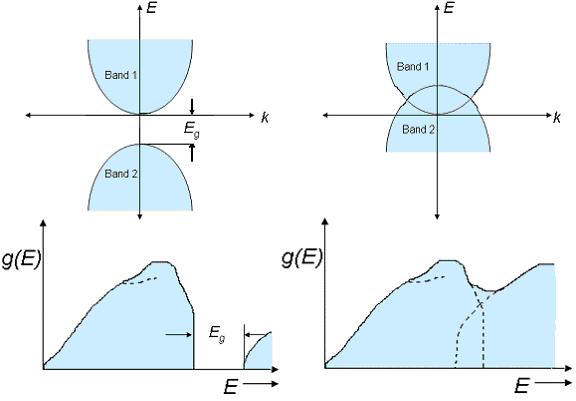
Figure \(\PageIndex{2}\)\(^{[1]}\) The left hand side shows a two-band diagram and a DOS vs.\(E\) plot for no band overlap. The right hand side shows a two-band diagram and a DOS vs. \(E\) plot for the case when there is a band overlap.
In simple metals the DOS can be calculated for most of the energy band, using:
\[ g(E) = \dfrac{1}{2\pi^2}\left( \dfrac{2m^*}{\hbar^2} \right)^{3/2} E^{1/2}\nonumber\]
however when we reach energies near the top of the band we must use a slightly different equation. To derive this equation we can consider that the next band is \(Eg\) ev below the minimum of the first band\(^{[1]}\). This is illustrated in the upper left plot in Figure \(\PageIndex{2}\). The energy of this second band is: \(E_2(k) =E_g-\dfrac{\hbar^2k^2}{2m^{\ast}}\). Now we can derive the density of states in this region in the same way that we did for the rest of the band and get the result:
\[ g(E) = \dfrac{1}{2\pi^2}\left( \dfrac{2|m^{\ast}|}{\hbar^2} \right)^{3/2} (E_g-E)^{1/2}\nonumber\]
Solving for the DOS in the other dimensions will be similar to what we did for the waves. i.e. for 2-D we would consider an area element in \(k\)-space \((k_x, k_y)\), and for 1-D a line element in \(k\)-space \((k_x)\). Figure \(\PageIndex{3}\) lists the equations for the density of states in 4 dimensions, (a quantum dot would be considered 0-D), along with corresponding plots of DOS vs. energy. Figure \(\PageIndex{4}\) plots DOS vs. energy over a range of values for each dimension and super-imposes the curves over each other to further visualize the different behavior between dimensions.
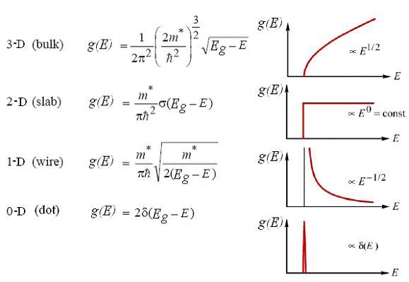
Figure \(\PageIndex{3}\)\(^{[4]}\)
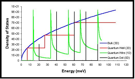
Figure \(\PageIndex{4}\)\(^{[3]}\)
References
- Sachs, M., Solid State Theory, (New York, McGraw-Hill Book Company, 1963),pp159-160;238-242.
- Omar, Ali M., Elementary Solid State Physics, (Pearson Education, 1999), pp68- 75;213-215.
- Semiconductor Physics (online) http://britneyspears.ac/physics/dos/dos.htm
- Density of States (online) www.ecse.rpi.edu/~schubert/Course-ECSE-6968%20Quantum%20mechanics/Ch12%20Density%20of%20states.pdf
Contributors and Attributions
ContribMSE5317