Thermocouples
- Page ID
- 325
\( \newcommand{\vecs}[1]{\overset { \scriptstyle \rightharpoonup} {\mathbf{#1}} } \)
\( \newcommand{\vecd}[1]{\overset{-\!-\!\rightharpoonup}{\vphantom{a}\smash {#1}}} \)
\( \newcommand{\dsum}{\displaystyle\sum\limits} \)
\( \newcommand{\dint}{\displaystyle\int\limits} \)
\( \newcommand{\dlim}{\displaystyle\lim\limits} \)
\( \newcommand{\id}{\mathrm{id}}\) \( \newcommand{\Span}{\mathrm{span}}\)
( \newcommand{\kernel}{\mathrm{null}\,}\) \( \newcommand{\range}{\mathrm{range}\,}\)
\( \newcommand{\RealPart}{\mathrm{Re}}\) \( \newcommand{\ImaginaryPart}{\mathrm{Im}}\)
\( \newcommand{\Argument}{\mathrm{Arg}}\) \( \newcommand{\norm}[1]{\| #1 \|}\)
\( \newcommand{\inner}[2]{\langle #1, #2 \rangle}\)
\( \newcommand{\Span}{\mathrm{span}}\)
\( \newcommand{\id}{\mathrm{id}}\)
\( \newcommand{\Span}{\mathrm{span}}\)
\( \newcommand{\kernel}{\mathrm{null}\,}\)
\( \newcommand{\range}{\mathrm{range}\,}\)
\( \newcommand{\RealPart}{\mathrm{Re}}\)
\( \newcommand{\ImaginaryPart}{\mathrm{Im}}\)
\( \newcommand{\Argument}{\mathrm{Arg}}\)
\( \newcommand{\norm}[1]{\| #1 \|}\)
\( \newcommand{\inner}[2]{\langle #1, #2 \rangle}\)
\( \newcommand{\Span}{\mathrm{span}}\) \( \newcommand{\AA}{\unicode[.8,0]{x212B}}\)
\( \newcommand{\vectorA}[1]{\vec{#1}} % arrow\)
\( \newcommand{\vectorAt}[1]{\vec{\text{#1}}} % arrow\)
\( \newcommand{\vectorB}[1]{\overset { \scriptstyle \rightharpoonup} {\mathbf{#1}} } \)
\( \newcommand{\vectorC}[1]{\textbf{#1}} \)
\( \newcommand{\vectorD}[1]{\overrightarrow{#1}} \)
\( \newcommand{\vectorDt}[1]{\overrightarrow{\text{#1}}} \)
\( \newcommand{\vectE}[1]{\overset{-\!-\!\rightharpoonup}{\vphantom{a}\smash{\mathbf {#1}}}} \)
\( \newcommand{\vecs}[1]{\overset { \scriptstyle \rightharpoonup} {\mathbf{#1}} } \)
\(\newcommand{\longvect}{\overrightarrow}\)
\( \newcommand{\vecd}[1]{\overset{-\!-\!\rightharpoonup}{\vphantom{a}\smash {#1}}} \)
\(\newcommand{\avec}{\mathbf a}\) \(\newcommand{\bvec}{\mathbf b}\) \(\newcommand{\cvec}{\mathbf c}\) \(\newcommand{\dvec}{\mathbf d}\) \(\newcommand{\dtil}{\widetilde{\mathbf d}}\) \(\newcommand{\evec}{\mathbf e}\) \(\newcommand{\fvec}{\mathbf f}\) \(\newcommand{\nvec}{\mathbf n}\) \(\newcommand{\pvec}{\mathbf p}\) \(\newcommand{\qvec}{\mathbf q}\) \(\newcommand{\svec}{\mathbf s}\) \(\newcommand{\tvec}{\mathbf t}\) \(\newcommand{\uvec}{\mathbf u}\) \(\newcommand{\vvec}{\mathbf v}\) \(\newcommand{\wvec}{\mathbf w}\) \(\newcommand{\xvec}{\mathbf x}\) \(\newcommand{\yvec}{\mathbf y}\) \(\newcommand{\zvec}{\mathbf z}\) \(\newcommand{\rvec}{\mathbf r}\) \(\newcommand{\mvec}{\mathbf m}\) \(\newcommand{\zerovec}{\mathbf 0}\) \(\newcommand{\onevec}{\mathbf 1}\) \(\newcommand{\real}{\mathbb R}\) \(\newcommand{\twovec}[2]{\left[\begin{array}{r}#1 \\ #2 \end{array}\right]}\) \(\newcommand{\ctwovec}[2]{\left[\begin{array}{c}#1 \\ #2 \end{array}\right]}\) \(\newcommand{\threevec}[3]{\left[\begin{array}{r}#1 \\ #2 \\ #3 \end{array}\right]}\) \(\newcommand{\cthreevec}[3]{\left[\begin{array}{c}#1 \\ #2 \\ #3 \end{array}\right]}\) \(\newcommand{\fourvec}[4]{\left[\begin{array}{r}#1 \\ #2 \\ #3 \\ #4 \end{array}\right]}\) \(\newcommand{\cfourvec}[4]{\left[\begin{array}{c}#1 \\ #2 \\ #3 \\ #4 \end{array}\right]}\) \(\newcommand{\fivevec}[5]{\left[\begin{array}{r}#1 \\ #2 \\ #3 \\ #4 \\ #5 \\ \end{array}\right]}\) \(\newcommand{\cfivevec}[5]{\left[\begin{array}{c}#1 \\ #2 \\ #3 \\ #4 \\ #5 \\ \end{array}\right]}\) \(\newcommand{\mattwo}[4]{\left[\begin{array}{rr}#1 \amp #2 \\ #3 \amp #4 \\ \end{array}\right]}\) \(\newcommand{\laspan}[1]{\text{Span}\{#1\}}\) \(\newcommand{\bcal}{\cal B}\) \(\newcommand{\ccal}{\cal C}\) \(\newcommand{\scal}{\cal S}\) \(\newcommand{\wcal}{\cal W}\) \(\newcommand{\ecal}{\cal E}\) \(\newcommand{\coords}[2]{\left\{#1\right\}_{#2}}\) \(\newcommand{\gray}[1]{\color{gray}{#1}}\) \(\newcommand{\lgray}[1]{\color{lightgray}{#1}}\) \(\newcommand{\rank}{\operatorname{rank}}\) \(\newcommand{\row}{\text{Row}}\) \(\newcommand{\col}{\text{Col}}\) \(\renewcommand{\row}{\text{Row}}\) \(\newcommand{\nul}{\text{Nul}}\) \(\newcommand{\var}{\text{Var}}\) \(\newcommand{\corr}{\text{corr}}\) \(\newcommand{\len}[1]{\left|#1\right|}\) \(\newcommand{\bbar}{\overline{\bvec}}\) \(\newcommand{\bhat}{\widehat{\bvec}}\) \(\newcommand{\bperp}{\bvec^\perp}\) \(\newcommand{\xhat}{\widehat{\xvec}}\) \(\newcommand{\vhat}{\widehat{\vvec}}\) \(\newcommand{\uhat}{\widehat{\uvec}}\) \(\newcommand{\what}{\widehat{\wvec}}\) \(\newcommand{\Sighat}{\widehat{\Sigma}}\) \(\newcommand{\lt}{<}\) \(\newcommand{\gt}{>}\) \(\newcommand{\amp}{&}\) \(\definecolor{fillinmathshade}{gray}{0.9}\)This page provides a fundamental discussion of what a thermocouple is and how it works. A thermocouple is a temperature measuring device that can operate in a wide range of temperature. It is created by joining two dissimilar metal and/or semiconductor wires together. Thermocouples are inexpensive to make. However, they have limited accuracy.
Introduction
A thermocouple is a device, joined together from two dissimilar metal and/or semiconductor wires, used for measuring temperatures. A thermocouple is not an absolute temperature measuring device. Instead, it is a device that responds to temperature difference between test environment and reference point, that produces a potential difference as the output. Incidentally, the potential difference is proportional to temperature difference between test environment and reference point, and is based on thermocouple materials. The output voltage allows us to backtrack and determine the temperature difference, and ultimately the temperature in test environment.
The advantage of measuring temperature with thermocouples is that thermocouples are able to be used in extreme environments, where typical thermometers would be unsuitable for use. For example, the K type thermocouple (chromel-alumel) operates from -269 degree to 1260 degree C, in non-oxidizing atmosphere.
Seebeck Effect
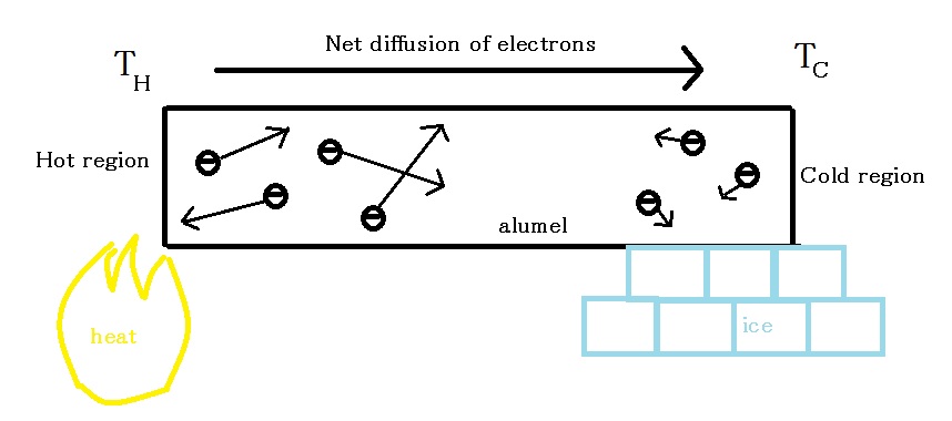
To understand how thermocouples work, first we must look at the Seebeck effect. The Seebeck effect is a phenomenon where a temperature gradient along a material produces a voltage going down from hotter region to colder region. To visualize this phenomenon, consider the alumel wire in Figure \(\PageIndex{1}\) below.

Thermal energy in hot region causes electrons in the vicinity to be more energetic than electrons in cold region. The average energy for electrons is described by the equation
\[E(T) = \dfrac{3}{5}E_{F}\left[1+\dfrac{5\pi ^{2}}{12}\left(\dfrac{k_{B}T}{E_{F}}\right)^{2}\right] \label{1}\]
where
- \(E_{F}\) is the specific material's Fermi energy,
- \(k_{B}\) is Boltzmann's constant, and
- \(T\) is absolute temperature.
From the above energy equation, we see that for a given material, higher temperature leads to higher average energy of electron. This results in energetic electrons in the hot region having higher velocities and diffusing into the cold region. Diffusion continues to take place until the electric field produced by charge imbalance grows strong enough to stop further diffusion. See Figure \(\PageIndex{2}\) for an illustration.

Since electrons diffused to the cold region, the hot region has become electron-deficient and positively charged. The cold region, on the other hand, has become electron-rich and negatively charged. Therefore, a potential difference exists going down from hot region to cold region. This potential difference is produced by temperature difference in the wire. In a small range of temperature difference, the potential and temperature difference are related by
\[\Delta V = S\Delta T \label{2}\]
where \(S\) is Seebeck coefficient, which is dependent on materials. \(S\) is essentially constant in small temperature ranges. However, for large \(ΔT\), \(S\) has been found to vary with temperature. And the Seebeck effect becomes
\[\Delta V = S(T) \Delta T \label{3}\]
where
\[ S(T)= -\dfrac{\pi ^{2}k_{B}^{2}T}{2eE_{F}} \label{4}\]
\(k_{B}\) is Boltzmann's constant, e is charge of an electron, \(E_{F}\) is the specific material's Fermi energy, and \(T\) is absolute temperature. The negative sign is canceled out with the negative charge of electron.
| Material | Seebeck coefficient, 298 K (µV/K) |
|---|---|
| K-type: chromel-alumel | 40 |
| J-type: iron-constantan | 51 |
| T-type: copper-constantan | 40 |
| E-type: chromel-constantan | 62 |
| N-type: nicrosil-nisil | 27 |
Concept of Thermocouples
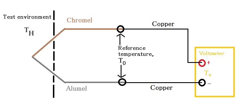
A thermocouple is composed of two dissimilar metal and/or semiconductor wires joined together. To use a thermocouple, we place the junction in the test environment and keep the two ends outside test environment at a reference temperature. Figure \(\PageIndex{3}\) demonstrates the proper setup for using a thermocouple.

In the above setup, as \(T_{H}\) increases, electrons diffuse away from test environment along both chromel and alumel wires. This creates a positive potential in the chromel-alumel junction and negative potentials at the two reference points. Because chromel and alumel are different materials and have different Seebeck coefficients, the voltage at the two reference points are also different. By measuring the voltage across these two ends, we would be able to determine the temperature difference, \(\Delta T\), between reference point and test environment. It is extremely important to keep the two ends of a thermocouple at the same, known temperature. This can be done by submerging the two reference points in a mixture bath of ice and water (273 K), for example. Because thermocouples only give us the \(\Delta T\) value between reference temperature and \(T_{H}\), if we do not know the reference temperature we would be unable to determine \(T_{H}\). In addition, if reference temperatures at the two ends are different, we would be measuring either too high or too low voltage on one side. Assuming that \(T_{0}\) is different from \(T_{v}\), Seebeck effect also exists in the copper wires connecting thermocouple to voltmeter. However, both copper wires have the same Seebeck coefficient and \(\Delta T\) values. Therefore they produce no change in the voltage across the two ends of thermocouple.
Disadvantages of and Concerns about Measuring Temperature with Thermocouple
Thermocouples are inexpensive, durable, and suitable to function over wide temperature ranges. However, they have limited accuracy.
Temperature measurement with a thermocouple relies on using predetermined Seebeck coefficients for the thermocouple and on the measured output voltage. However, impurities and defects introduced during manufacturing can cause thermocouples produced in the same batch to have varied Seebeck coefficients. For thermodynamic reasons, materials with high purity are very susceptible to contamination. Therefore, some thermocouple manufacturers deliberately introduce controlled amounts of impurities to thermocouples so that they would be more protected from further contamination during use. Because the output voltages across thermocouples are usually on the order of microvolt, there is also an issue with large uncertainty when converting measured voltage to temperature. So in experiments where precise and accurate readings are required, it would be good to consider other temperature measuring devices such as the silicon band-fgap temperature sensor and resistance thermometer, which have higher accuracy. Another issue with thermal couple is the age hardening effect. Thermocouples are typically placed into the furnace at the thermocouple junction and kept in ambient condition at the two ends. Inside the furnace, temperature is high and the environment can be quite reactive. Such conditions can lead to age hardening of the part inside furnace and make the thermocouple wires become inhomogeneous. Inhomogeneity causes Seebeck coefficients to change, which affect the output voltage readings. To minimize this source of error when using thermocouple, it is important to check the thermocouple wires throughout experiment. This can be done by simply looking at the sample's macroscopic optical properties. If you see that a part of the thermocouple inside the furnace looks different from the region outside the furnace, try to push the thermocouple further into the furnace. This puts the age hardened section deeper into the furnace, removing temperature gradient along the aged section so that it does not produce any Seebeck effect.
Questions
- Why do we use thermocouples instead of regular thermometers?
- Why do thermocouples have to be made from two different materials?
Answers
- Regular thermometers cannot withstand very low or very high temperatures. They typically measure between -30 degree and 200 degree Celsius. Although thermometers that measure significantly beyond this range do exist, they are usually quite expensive. Thermocouples are inexpensive devices that allow us to measure system temperatures in extreme conditions. A K-type thermocouple probe that measures from -100 to 1250 degree C can be bought for just $10.
- When a thermocouple made from two similar materials is heated to create a temperature gradient along each wire, according to Seebeck effect, voltage across each wire would be the same. These voltages would cancel each other out and we would be measuring a zero voltage across the two wires at all temperatures. This also means we would not be able to measure \(ΔT\) or the temperature at the junction.
References
- R. E. Hummel, Electronic Properties of Materials, 4th ed. New York: Springer, 2012.
- J.W. Davisson. Thermoelectricity. Fe. Belvoir: Defense Technical Information Center, 1962.
- S. Kasap. Thermoelectric Effects in Metals: Thermocouples. Department of Electrical Engineering. University of Saskatchewan, Canada. An e-Booklet. 2001.

