6.1: Images as Two-Dimensional Signals

Last updated
Save as PDF

Page ID: 14802

\( \newcommand{\vecs}[1]{\overset { \scriptstyle \rightharpoonup} {\mathbf{#1}} } \) \( \newcommand{\vecd}[1]{\overset{-\!-\!\rightharpoonup}{\vphantom{a}\smash {#1}}} \)\(\newcommand{\id}{\mathrm{id}}\) \( \newcommand{\Span}{\mathrm{span}}\) \( \newcommand{\kernel}{\mathrm{null}\,}\) \( \newcommand{\range}{\mathrm{range}\,}\) \( \newcommand{\RealPart}{\mathrm{Re}}\) \( \newcommand{\ImaginaryPart}{\mathrm{Im}}\) \( \newcommand{\Argument}{\mathrm{Arg}}\) \( \newcommand{\norm}[1]{\| #1 \|}\) \( \newcommand{\inner}[2]{\langle #1, #2 \rangle}\) \( \newcommand{\Span}{\mathrm{span}}\) \(\newcommand{\id}{\mathrm{id}}\) \( \newcommand{\Span}{\mathrm{span}}\) \( \newcommand{\kernel}{\mathrm{null}\,}\) \( \newcommand{\range}{\mathrm{range}\,}\) \( \newcommand{\RealPart}{\mathrm{Re}}\) \( \newcommand{\ImaginaryPart}{\mathrm{Im}}\) \( \newcommand{\Argument}{\mathrm{Arg}}\) \( \newcommand{\norm}[1]{\| #1 \|}\) \( \newcommand{\inner}[2]{\langle #1, #2 \rangle}\) \( \newcommand{\Span}{\mathrm{span}}\)\(\newcommand{\AA}{\unicode[.8,0]{x212B}}\)

Images are captured by cameras containing matrices of charge-coupled devices (CCD) or similar semi-conductors that can turn photons into electrical signals. These matrices can be read out pixel by pixel and turned into digital values, for example an array of 640 by 480 three-byte tuples corresponding to the red, green, and blue (RGB) components the camera has seen. An example of such data, for simplicity only one color channel, is shown in Figure 6.1.1.

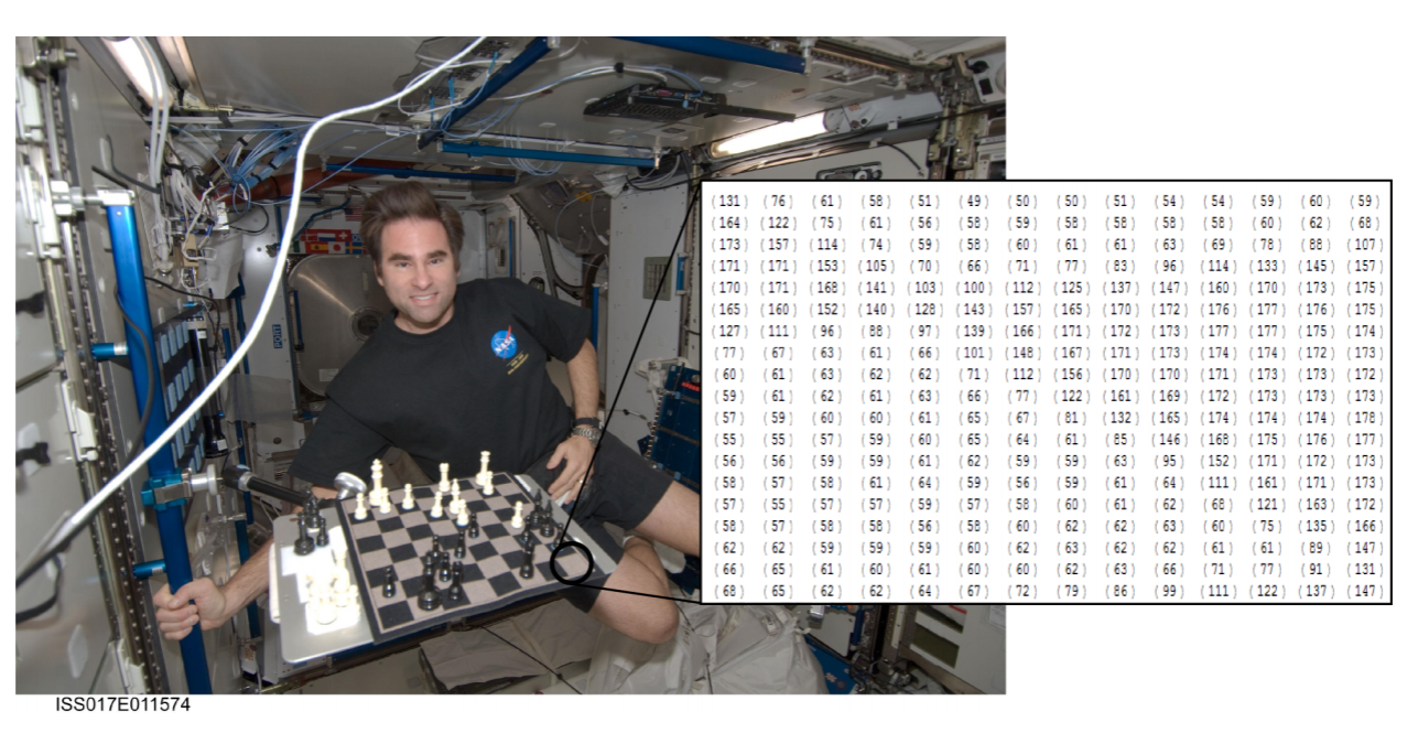
Figure \(\PageIndex{1}\): A chessboard floating inside the ISS, astronaut Gregory Chamitoff. The inset shows a sample of the actual data recorded by the image sensor. One can clearly recognize the contours of the white tile.

Looking at the data clearly reveals the white tile within the black tiles at the lower-right corner of the chessboard. Higher values correspond to brighter colors (white) and lower values to darker colors. We also observe that although the tiles have to have the same color, the actual values differ quite a bit. It might make sense to think about these values much like we would do if the data would be 1D signal: taking the “derivative”, e.g., along the horizontal rows, would indicate areas of big changes, whereas the “frequency” of an image would indicate how quickly values change. Areas with smooth gradients, e.g., black and white tiles, would then have low frequencies, whereas areas with strong gradients, would contain high frequency information.

This language opens the door to a series of signal processing concepts, such as low-pass filters (supressing high frequency information), high-pass filters (suppressing low frequency information), or band-pass filters (letting only a range of frequencies pass), analysis of the frequency spectrum of the image (the distribution of content at different frequencies), or “convolving” the image with another two-dimensional function. The next sections will provide both an intuition of what kind of meaningful information is hidden in such abstract data and provide concrete examples of signal processing techniques that make this information appear.