6.2: From Signals to Information

Last updated
Save as PDF

Page ID: 14803

\( \newcommand{\vecs}[1]{\overset { \scriptstyle \rightharpoonup} {\mathbf{#1}} } \) \( \newcommand{\vecd}[1]{\overset{-\!-\!\rightharpoonup}{\vphantom{a}\smash {#1}}} \)\(\newcommand{\id}{\mathrm{id}}\) \( \newcommand{\Span}{\mathrm{span}}\) \( \newcommand{\kernel}{\mathrm{null}\,}\) \( \newcommand{\range}{\mathrm{range}\,}\) \( \newcommand{\RealPart}{\mathrm{Re}}\) \( \newcommand{\ImaginaryPart}{\mathrm{Im}}\) \( \newcommand{\Argument}{\mathrm{Arg}}\) \( \newcommand{\norm}[1]{\| #1 \|}\) \( \newcommand{\inner}[2]{\langle #1, #2 \rangle}\) \( \newcommand{\Span}{\mathrm{span}}\) \(\newcommand{\id}{\mathrm{id}}\) \( \newcommand{\Span}{\mathrm{span}}\) \( \newcommand{\kernel}{\mathrm{null}\,}\) \( \newcommand{\range}{\mathrm{range}\,}\) \( \newcommand{\RealPart}{\mathrm{Re}}\) \( \newcommand{\ImaginaryPart}{\mathrm{Im}}\) \( \newcommand{\Argument}{\mathrm{Arg}}\) \( \newcommand{\norm}[1]{\| #1 \|}\) \( \newcommand{\inner}[2]{\langle #1, #2 \rangle}\) \( \newcommand{\Span}{\mathrm{span}}\)\(\newcommand{\AA}{\unicode[.8,0]{x212B}}\)

Unfortunately, many phenomena that often have very different or even opposite meaning look very similar when looking at the low-level signal. For example, drastic changes in color values do not necessarily mean that the color of a surface indeed has changed. Similar patterns are generated by depth discontinuities, specular highlights, changing lighting conditions, or surface orientation changes. These examples are illustrated in Figure 6.2.1 and make computer vision a hard problem.

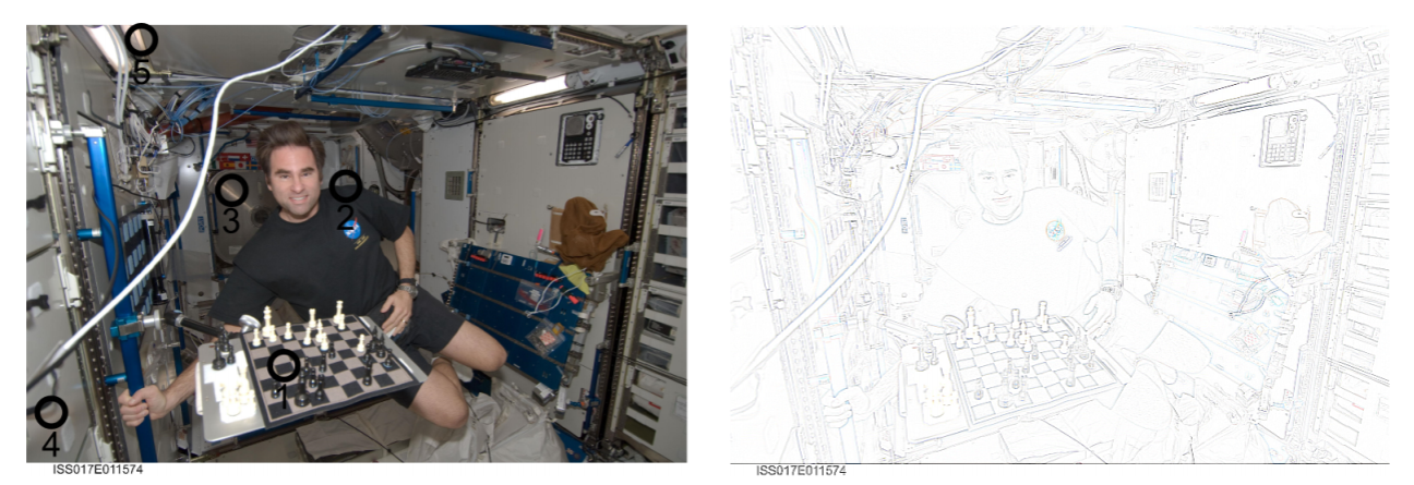
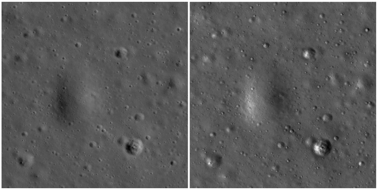
Figure \(\PageIndex{1}\): Inside of the international space station (left), highlighted areas in which pixel values change drastically (right). Underlying effects that produce similar responses: change in surface properties (1), depth discontinuities (2), specular highlights (3), changing lighting conditions such as shadows (4), or surface orientation changes (5).

This example illustrates that signals alone are not sufficient to understand a phenomenon, but require context. Here, the context does not only refer to surrounding signals, but also high-level conceptional knowledge such as the fact that light sources create shadows and specular highlights, that objects in the front appear larger, and so on. How important such conceptional knowledge is, is illustrated by Figure 6.2.1.

Both images show an identical landscape that once appears to be speckled with craters, once with bubble-like hills. At first glance, both scenes are illuminated from the left, suggesting a change in the landscape. Once information that the sun is illuminating one picture from the left and the other from the right, however, it becomes clear that the craters are simply differently illuminated and what we perceive as bumps eventually turns back into craters.

Figure \(\PageIndex{2}\): Picture of the Apollo 15 landing site during different times of the day. The landscape is identical, but appears to be speckled with craters (lift) or hills (right). Knowing that the sun is illuminating the scene from the left and right, respectively, does explain this effect. Image credit: NASA/GSFC/Arizona State University.

More surprisingly, conceptual knowledge is often sufficient to make up for the lack of low-level cues in an image. An example is shown in Figure 6.4. Here, a Dalmatian dog can be clearly recognized despite absence of cues for its outline, simply by extrapolating its appearance and pose from conceptual knowledge.

These examples illustrate both the advantages and drawbacks of a signal processing approach. While an algorithm will detect interesting signals even there where we don’t see, or don’t expect them (due to conceptional bias), image understanding not only requires low-level processing, but intelligent combination of the low-level cue’s spatial relationship and conceptual knowledge about the world.