6.3: Basic Image Operations

Basic image operations can be thought of as a filter that operates in the frequency or in the space (color) domain. Although most filters directly operate in the color domain, knowing how they affect the frequency domain is helpful in understanding the filter’s function. For example, a filter that is supposed to highlight edges, such as shown in Figure 6.2.1 should suppress low frequencies, i.e., areas in which the color values do not change much, and amplify high-frequency information, i.e., areas in which the color values change quickly. The goal of this section is to provide a basic understanding of how basic image processing operation works. The methods presented here, while still valid, have been superseded by more sophisticated implementations that are widely available as software packages or within desktop graphic software.

Figure \(\PageIndex{1}\): The image of a Dalmatian dog can be clearly recognized by most spectators even though low-level cues such as edges are only present for ears, chin and parts of the legs. The contours of the animals are highlighted in a flipped version of the image in the inset.

6.3.1. Convolution-based filters

A filter can be implemented using the convolution operator that convolves function f() with function g().

\[f(x) \star g(x)=\int_{-\infty }^{\infty }f(\tau )g(x-\tau )d\tau \]

We then call function g() a filter . As will become more clear further below, the convolution literally shifts the function g() across the function f() while multiplying the two. As images are discrete signals, the convolution is usually discrete

\[f\left [ x \right ]\star g[x]=\sum_{i=-\infty }^{\infty }f[i]g[x-i]\]

For 2D signals, like images, the convolution is also two-dimensional:

\[f[x,y]\star g[x,y]=\sum_{i=-\infty }^{\infty }\sum_{j=-\infty }^{\infty }f[i,j]g[x-i,y-j]\]

Although we have defined the convolution from negative infinity to infinity, both images and filters are usually finite. Images are constrained by their resolution, and filters are usually much smaller than the images themselves. Also, the convolution is commutative, therefore (6.3.3) is equivalent to

\[f[x,y]\star g[x,y]=\sum_{i=-\infty }^{\infty }\sum_{j=-\infty }^{\infty }f[x-i,y-j]g[i,j]\]

Gaussian smoothing

A very important filter is the Gaussian filter. It is shaped like the Gaussian bell function and can be easily stored in a 2D matrix. Implementing a Gaussian filter is surprisingly simple, e.g., such as

\[g(x,y)=\frac{1}{10}\begin{pmatrix}
1 & 1 & 1\\
1& 2 &1 \\
1 & 1 & 1
\end{pmatrix}\]

Using this filter in Equation 6.3.4 on an infinitely large image f() leads to

\[f[x,y]\star g[x,y]=\sum_{i=-1 }^{1 }\sum_{j=-1 }^{1 }f[x-i,y-j]g[i,j]\]

(assuming g(0, 0) addresses the center of the matrix). What now happens is that each pixel f(x, y) becomes the average of that of its neighbors, with its previous value weighted twice (as g(0, 0) = 0.2) that of their neighbors. More concretely,

\[f(x,y)=llf(x+1,y+1)g(-1,-1)+f(x+1,y)g(-1,0)+f(x+1,y-1)g(-1,1)+f(x,y+1)g(0,−1) +f(x,y)g(0,0) +f(x,y−1)g(0,1)
+f(x−1,y+1)g(1,−1) +f(x−1,y)g(1,0) +f(x−1,y−1)g(1,1)\]

Doing this for all x and all y literally corresponds to sliding the filter g() along the image.

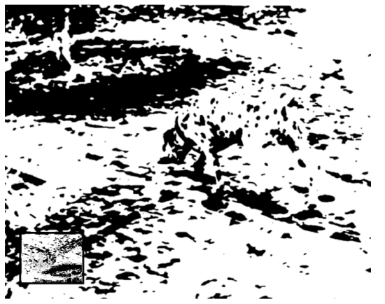
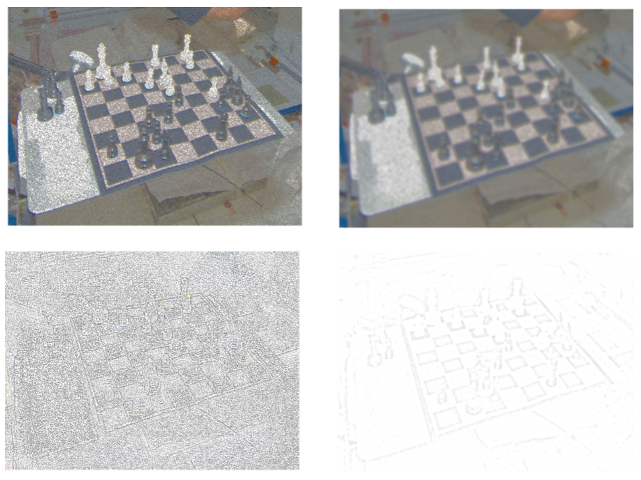
An example of filter g(x, y) in action is shown in Figure 6.3.2. The filter acts as a low-pass filter , suppressing high frequency components. Indeed, noise in the image is suppressed, leading also to a smoother edge image, which is shown underneath.

Edge detection

Edge detection can be achieved using another convolution-based filter, the Sobel kernel

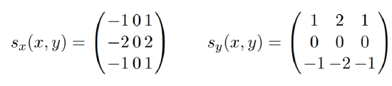
Here, s_x(x, y) can be used to detect vertical edges, whereas s_y(x, y) highlights horizontal edges. Edge detectors, such as the Canny edge detector therefore run at least two of such filters over an image to detect both horizontal and vertical edges.

Figure \(\PageIndex{2}\): A noisy image before (top left) and after filtering with a Gaussian kernel (top right). Corresponding edge images are shown underneath.

Difference of Gaussians

An alternative method for detecting edges is the Difference of Gaussians (DoG) method. The idea is to subtract two images that have each been filtered using a Gaussian kernel with different width. Both filters supress high-frequency information and their difference therefore leads to a band-pass filtered signal, from which both low and high frequencies have been removed. As such, a DoG filter acts as a capable edge detection algorithm. Here, one kernel is usually four to five times wider than the other, therefore acting as a much stronger filter.

Differences of Gaussians can also be used to approximate the Laplacian of Gaussian, i.e., the sum of the second derivatives of a Gaussian kernel. Here, one kernel is roughly 1.6 times wider than the other. The band-pass characteristic of DoG and LoGs are important as they highlight high-frequency information such as edges, yet suppress high-frequency noise in the image.

6.3.2. Threshold-based operations

In order to find objects with a certain color or edge intensity, thresholding an image will lead to a binary image that contains “true-false” regions that fit the desired criteria. Thresholds make use of operators like >, <, ≤, ≥ and combinations thereof. There also exist adaptive versions that would adapt the thresholds locally, e.g., to make up for changing lighting conditions.

Albeit thresholding is deceptively simple, finding correct threshold values is a hard problem. In particular, actual pixel values change drastically with changing lighting conditions and there is no such thing as “red” or “green” when inspecting the actual values under different conditions.

Figure \(\PageIndex{3}\): Examples of morphological operators erosion and dilation and combinations thereof.

6.3.3. Morphological Operations

Another class of filters are morphological operators which consists of a kernel describing the structure of the operation (this can be as simple as an identity matrix) and a rule on how to change a pixel value based on the values in the neighborhood defined by the kernel.

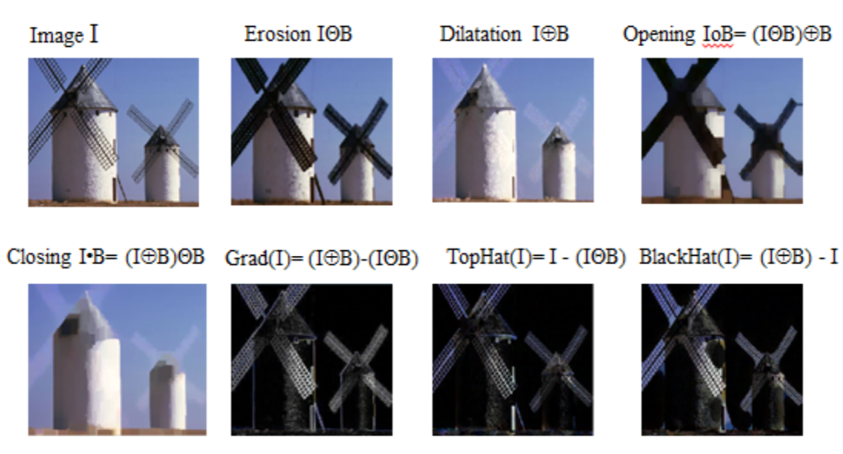
Important morphological operators are erosion and dilation. The erosion operator assigns a pixel value with the minimum value that it can find in the neighborhood defined by the kernel. The dilation operator assigns a pixel value with the maximum value it can find in the neighborhood defined by the kernel. This is useful, e.g., to fill holes in a line or remove noise. A dilation followed by an erosion is known as a “Closing” and an erosion followed by a dilation as an “Opening”. Subtracting erosed and dilated images from each other can also serve as an edge detector. Examples of such operators are shown in Figure 6.3.3.