7.1: Integration of Univariate Functions

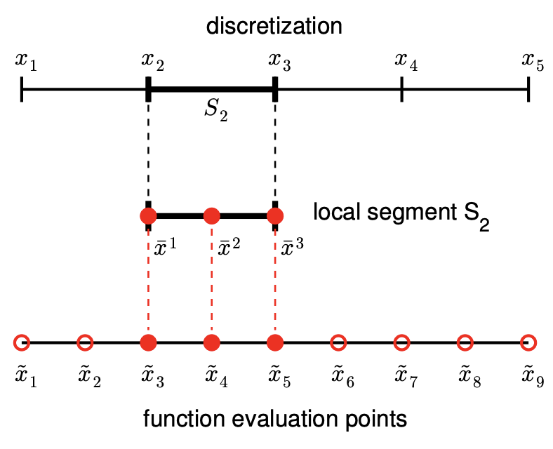
Our objective is to approximate the value of the integral \[ I=\int_{a}^{b} f(x) d x,\] for some arbitrary univariate function \(f(x)\). Our approach to this integration problem is to approximate function \(f\) by an interpolant \(\mathcal{I} f\) and to exactly integrate the interpolant, i.e. \[\tag{7.1} I=\sum_{i=1}^{N-1} \int_{S_{i}} f(x) d x \approx \sum_{i=1}^{N-1} \int_{S_{i}}(\mathcal{I} f)(x) d x \equiv I_{h}\] Recall that in constructing an interpolant, we discretize the domain \([a, b]\) into \(N-1\) non-overlapping segments, delineated by segmentation points \(x_{i}, i=1, \ldots, N\), as illustrated in Figure \(7.1^{1}\) Then, we construct a polynomial interpolant on each segment using the function values at the local interpolation points, \(\bar{x}^{m}, m=1, \ldots, M\). These local interpolation points can be mapped to global function evaluation points, \(\tilde{x}_{i}, i=1, \ldots, N_{\text {eval }}\). The quality of the interpolant is dictated by its type and the segment length \(h\), which in turn governs the quality of the integral approximation, \(I_{h}\). The subscript \(h\) on \(I_{h}\) signifies that the integration is performed on a discretization with a segment length \(h\). This integration process takes advantage of the ease of integrating the polynomial interpolant on each segment.

Recalling that the error in the interpolation decreases with \(h\), we can expect the approximation of the integral \(I_{h}\) to approach the true integral \(I\) as \(h\) goes to 0 . Let us formally establish the relationship between the interpolation error bound, \(e_{\max }=\max _{i} e_{i}\), and the integration error,

\({ }^{1}\) For simplicity, we assume \(h\) is constant throughout the domain.

Figure 7.1: Discretization of a 1d domain into \(N-1\) (here \(N=5\) ) segments of length \(h\).

\(\left|I-I_{h}\right| .\) \[\begin{aligned} \left|I-I_{h}\right| &=\left|\sum_{i=1}^{N-1} \int_{S_{i}}(f(x)-(\mathcal{I} f)(x)) d x\right| \\ & \leq\left|\sum_{i=1}^{N-1} \int_{S_{i}}\right| f(x)-(\mathcal{I} f)(x)|d x| \\ & \leq\left|\sum_{i=1}^{N-1} \int_{S_{i}} e_{i} d x\right| \\ & \leq \sum_{i=1}^{N-1} e_{i} h \\ & \leq e_{\max } \sum_{i=1}^{N-1} h \\ &=(b-a) e_{\max } . \end{aligned}\] \[\begin{aligned} & \begin{aligned}&\leq \sum_{i=1} \int_{S_{i}} e_{i} d x \mid \\&\leq \sum_{i=1}^{N-1} e_{i} h \quad \text { (definition of } h \text { ) }\end{aligned} \end{aligned}\] (definition of \(e_{\max }\) )

We make a few observations. First, the global error in the integral is a sum of the local error contributions. Second, since all interpolation schemes considered in Section \(2.1\) are convergent \(\left(e_{\max } \rightarrow 0\right.\) as \(\left.h \rightarrow 0\right)\), the integration error also vanishes as \(h\) goes to zero. Third, while this bound applies to any integration scheme based on interpolation, the bound is not sharp; i.e., some integration schemes would display better convergence with \(h\) than what is predicted by the theory.

Recall that the construction of a particular interpolant is only dependent on the location of the interpolation points and the associated function values, \(\left(\tilde{x}_{i}, f\left(\tilde{x}_{i}\right)\right), i=1, \ldots, N_{\mathrm{eval}}\), where \(N_{\text {eval }}\) is the number of the (global) function evaluation points. As a result, the integration rules based on the interpolant is also only dependent on the function values at these \(N_{\text {eval }}\) points. Specifically, all integration rules considered in this chapter are of the form \[I_{h}=\sum_{i=1}^{N_{\text {eval }}} w_{i} f\left(\tilde{x}_{i}\right),\] where \(w_{i}\) are the weights associated with each point and are dependent on the interpolant from which the integration rules are constructed. In the context of numerical integration, the function evaluation points are called quadrature points and the associated weights are called quadrature weights. The quadrature points and weights together constitute a quadrature rule. Not too surprisingly considering the Riemann integration theory, the integral is approximated as a linear combination of the function values at the quadrature points.

Let us provide several examples of integration rules.

Example 7.1.1 rectangle rule, left

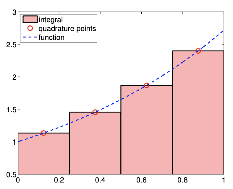
The first integration rule considered is a rectangle rule based on the piecewise-constant, leftendpoint interpolation rule considered in Example 2.1.1. Recall the interpolant over each segment is obtained by approximating the value of the function by a constant function that matches the value of the function at the left endpoint, i.e., the interpolation point is \(\bar{x}^{1}=x_{i}\) on segment \(S_{i}=\left[x_{i}, x_{i+1}\right]\). The resulting integration formula is \[I_{h}=\sum_{i=1}^{N-1} \int_{S_{i}}(\mathcal{I} f)(x) d x=\sum_{i=1}^{N-1} \int_{S_{i}} f\left(x_{i}\right) d x=\sum_{i=1}^{N-1} h f\left(x_{i}\right)\] where the piecewise-constant function results in a trivial integration. Recalling that the global function evaluation points, \(\tilde{x}_{i}\), are related to the segmentation points, \(x_{i}\), by \[\tilde{x}_{i}=x_{i}, \quad i=1, \ldots, N-1,\] we can also express the integration rule as \[I_{h}=\sum_{i=1}^{N-1} h f\left(\tilde{x}_{i}\right) .\] Figure 7.2(a) illustrates the integration rule applied to \(f(x)=\exp (x)\) over \([0,1]\) with \(N=5\). Recall that for simplicity we assume that all intervals are of the same length, \(h \equiv x_{i+1}-x_{i}, i=1, \ldots, N-1\).

Let us now analyze the error associated with this integration rule. From the figure, it is clear that the error in the integrand is a sum of the local errors committed on each segment. The local error on each segment is the triangular gap between the interpolant and the function, which has the length of \(h\) and the height proportional to \(f^{\prime} h\). Thus, the local error scales as \(f^{\prime} h^{2}\). Since there are \((b-a) / h\) segments, we expect the global integration error to scale as \[\left|I-I_{h}\right| \sim f^{\prime} h^{2}(b-a) / h \sim h f^{\prime} .\] More formally, we can apply the general integration error bound, Eq. (7.7), to obtain \[\left|I-I_{h}\right| \leq(b-a) e_{\max }=(b-a) h \max _{x \in[a, b]}\left|f^{\prime}(x)\right| .\] In fact, this bound can be tightened by a constant factor, yielding \[\left|I-I_{h}\right| \leq(b-a) \frac{h}{2} \max _{x \in[a, b]}\left|f^{\prime}(x)\right| .\]

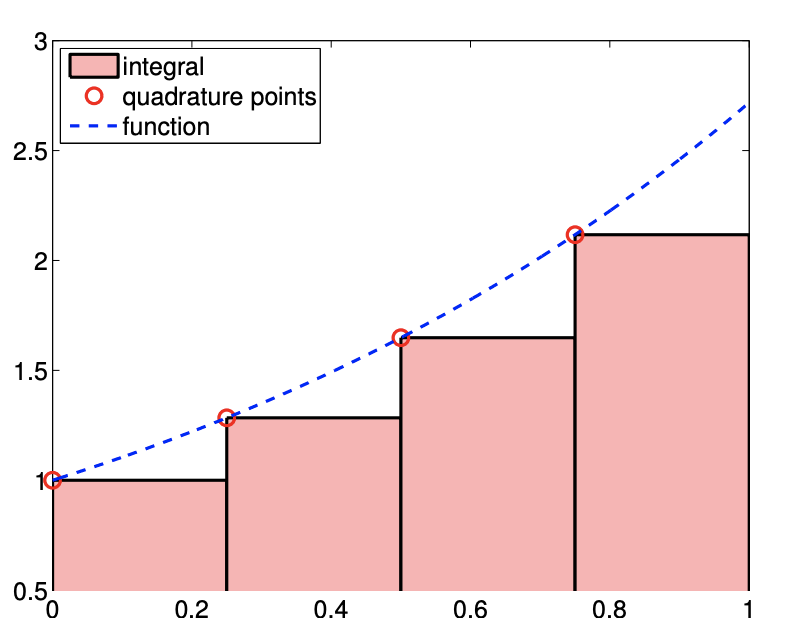
(a) integral

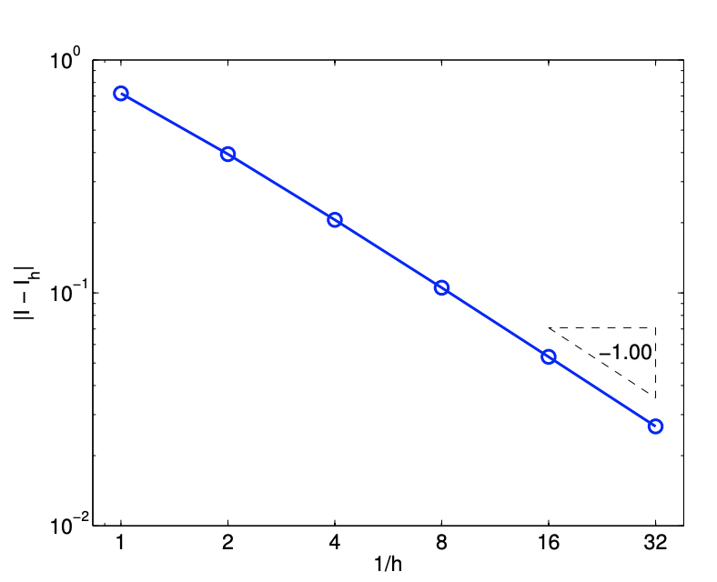
(b) error

Figure 7.2: Rectangle, left-endpoint rule.

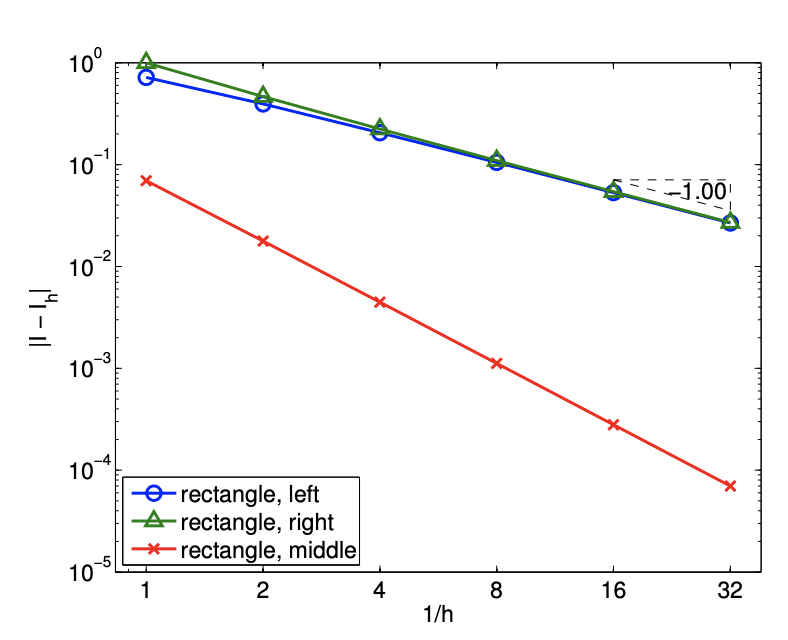
Figure 7.2(b) captures the convergence behavior of the scheme applied to the exponential function. As predicted by the theory, this integration rule is first-order accurate and the error scales as \(\mathcal{O}(h)\). Note also that the approximation \(I_{h}\) underestimates the value of \(I\) if \(f^{\prime}>0\) over the domain.

Before we proceed to a proof of the sharp error bound for a general \(f\), let us analyze the integration error directly for a linear function \(f(x)=m x+c\). In this case, the error can be expressed as \[\begin{aligned} \left|I-I_{h}\right| &=\sum_{i=1}^{N-1} \int_{S_{i}} f(x)-(\mathcal{I} f)(x) d x=\sum_{i=1}^{N-1} \int_{x_{i}}^{x_{i+1}}(m x-c)-\left(m x_{i}-c\right) d x \\ &=\sum_{i=1}^{N-1} \int_{x_{i}}^{x_{i+1}} m \cdot\left(x-x_{i}\right) d x=\sum_{i=1}^{N-1} \frac{1}{2} m\left(x_{i+1}-x_{i}\right)^{2} \\ &=\frac{1}{2} m h \sum_{i=1}^{N-1} h=\frac{1}{2} m h(b-a), \end{aligned}\] Note that the integral of \(m \cdot\left(x-x_{i}\right)\) over \(S_{i}\) is precisely equal to the area of the missing triangle, with the base \(h\) and the height \(m h\). Because \(m=f^{\prime}(x), \forall x \in[a, b]\), we confirm that the general error bound is correct, and in fact sharp, for the linear function. Let us now prove the result for a general \(f\).

Proof

By the fundamental theorem of calculus, we have \[f(x)-(\mathcal{I} f)(x)=\int_{x_{i}}^{x} f^{\prime}(\xi) d \xi, \quad x \in S_{i}=\left[x_{i}, x_{i+1}\right]\] Integrating the expression over segment \(S_{i}\) and using the Mean Value Theorem, \[\begin{aligned} \int_{S_{i}} f(x)-(\mathcal{I} f)(x) d x &=\int_{x_{i}}^{x_{i+1}} \int_{x_{i}}^{x} f^{\prime}(\xi) d \xi d x \\ &=\int_{x_{i}}^{x_{i+1}}\left(x-x_{i}\right) f^{\prime}(z) d x \\ & \leq \int_{x_{i}}^{x_{i+1}}\left|\left(x-x_{i}\right) f^{\prime}(z)\right| d x \\ & \leq\left(\int_{x_{i}}^{x_{i+1}}\left|x-x_{i}\right| d x\right) \max _{z \in\left[x_{i}, x_{i+1}\right]}\left|f^{\prime}(z)\right| \\ &=\frac{1}{2}\left(x_{i+1}-x_{i}\right)^{2} \max _{z \in\left[x_{i}, x_{i+1}\right]}\left|f^{\prime}(z)\right| \\ & \leq \frac{1}{2} h^{2} \max _{x \in\left[x_{i}, x_{i+1}\right]}\left|f^{\prime}(x)\right| . \end{aligned}\] (Mean Value Theorem, for some \(z \in\left[x_{i}, x\right]\) )

Summing the local contributions to the integral error, \[\left|I-I_{h}\right|=\left|\sum_{i=1}^{N-1} \int_{S_{i}} f(x)-(\mathcal{I} f)(x) d x\right| \leq \sum_{i=1}^{N-1} \frac{1}{2} h^{2} \max _{x \in\left[x_{i}, x_{i+1}\right]}\left|f^{\prime}(x)\right| \leq(b-a) \frac{h}{2} \max _{x \in[a, b]}\left|f^{\prime}(x)\right|\

Example 7.1.2 rectangle rule, right

This integration rule is based on the piecewise-constant, right-endpoint interpolation rule considered in Example 2.1.2, in which the interpolation point is chosen as \(\bar{x}^{1}=x_{i+1}\) on segment \(S_{i}=\left[x_{i}, x_{i+1}\right]\). This results in the integration formula \[I_{h}=\sum_{i=1}^{N-1} \int_{S_{i}}(\mathcal{I} f)(x) d x=\sum_{i=1}^{N-1} \int_{S_{i}} f\left(x_{i+1}\right) d x=\sum_{i=1}^{N-1} h f\left(x_{i+1}\right) .\] Recalling that global function evaluation points are related to the segmentation points by \(\tilde{x}_{i}=x_{i+1}\), \(i=1, \ldots, N-1\), we also have \[I_{h}=\sum_{i=1}^{N-1} h f\left(\tilde{x}_{i}\right) .\] While the form of the equation is similar to the rectangle rule, left, note that the location of the quadrature points \(\tilde{x}_{i}, i=1, \ldots, N-1\) are different. The integration process is illustrated in Figure 7.1.2

Figure 7.3: Rectangle, right-endpoint rule.

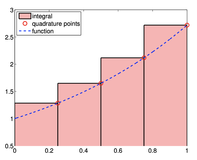
This rule is very similar to the rectangle rule, left. In particular, the integration error is bounded by \[\left|I-I_{h}\right| \leq(b-a) \frac{h}{2} \max _{x \in[a, b]}\left|f^{\prime}(x)\right| .\] The expression shows that the scheme is first-order accurate, and the rule integrates constant function exactly. Even though the error bounds are identical, the left- and right-rectangle rules in general give different approximations. In particular, the right-endpoint rule overestimates \(I\) if \(f^{\prime}>0\) over the domain. The proof of the error bound identical to that of the left-rectangle rule.

While the left- and right-rectangle rule are similar for integrating a static function, they exhibit fundamentally different properties when used to integrate an ordinary differential equations. In particular, the left- and right-integration rules result in the Euler forward and backward schemes, respectively. These two schemes exhibit completely different stability properties, which will be discussed in chapters on Ordinary Differential Equations.

Example 7.1.3 rectangle rule, midpoint

The third integration rule considered is based on the piecewise-constant, midpoint interpolation rule considered in Example 2.1.3. Choosing the midpoint \(\bar{x}^{1}=\left(x_{i}+x_{i+1}\right)\) as the interpolation point for each \(S_{i}=\left[x_{i}, x_{i+1}\right]\), the integration formula is given by \[I_{h}=\sum_{i=1}^{N-1} \int_{S_{i}}(\mathcal{I} f)(x) d x=\sum_{i=1}^{N-1} \int_{S_{i}} f\left(\frac{x_{i}+x_{i+1}}{2}\right) d x=\sum_{i=1}^{N-1} h f\left(\frac{x_{i}+x_{i+1}}{2}\right)\] Recalling that the global function evaluation point of the midpoint interpolation is related to the segmentation points by \(\tilde{x}_{i}=\left(x_{i}+x_{i+1}\right) / 2, i=1, \ldots, N-1\), the quadrature rule can also be expressed as \[\sum_{i=1}^{N-1} h f\left(\tilde{x}_{i}\right)\] The integration process is illustrated in Figure \(7.4(\mathrm{a}) .\)

(a) integral

(b) error

Figure 7.4: Rectangle, midpoint rule.

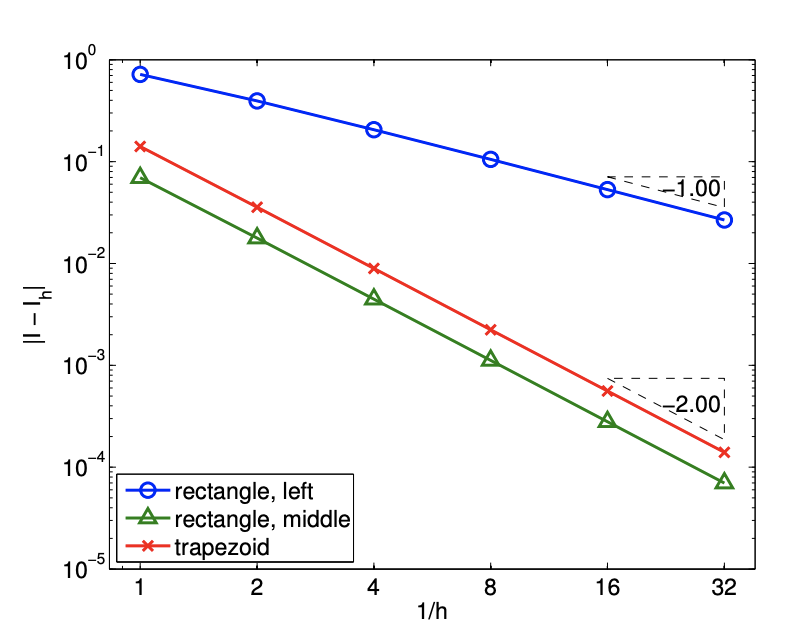
The error analysis for the midpoint rule is more involved than that of the previous methods. If we apply the general error bound, Eq. (7.7), along with the interpolation error bounds for the midpoint rule, we obtain the error bound of \[\left|I-I_{h}\right| \leq(b-a) e_{\max } \leq(b-a) \frac{h}{2} \max _{x \in[a, b]}\left|f^{\prime}(x)\right|\] However, this bound is not sharp. The sharp error bound for the rectangle, midpoint integration rule is given by \[\left|I-I_{h}\right| \leq \frac{1}{24}(b-a) h^{2} \max _{x \in[a, b]}\left|f^{\prime \prime}(x)\right|\] Thus, the rectangle, midpoint rule is second-order accurate. The higher accuracy and convergence rate of the midpoint rule are captured in the error convergence plot in Figure \(7.4(\mathrm{~b})\).

Before we prove the error bound for a general \(f\), let us show that the rectangle rule in fact integrates a linear function \(f(x)=m x+c\) exactly. The integration error for a linear function can be expressed as \[\begin{aligned} I-I_{h} &=\sum_{i=1}^{N-1} \int_{S_{i}} f(x)-(\mathcal{I} f)(x) d x=\sum_{i=1}^{N-1} \int_{x_{i}}^{x_{i+1}} f(x)-f\left(\frac{x_{i}+x_{i+1}}{2}\right) d x \\ &=\sum_{i=1}^{N-1} \int_{x_{i}}^{x_{i+1}}(m x+c)-\left(m\left(\frac{x_{i}+x_{i+1}}{2}\right)+c\right) d x \\ &=\sum_{i=1}^{N-1} \int_{x_{i}}^{x_{i+1}} m\left[x-\frac{x_{i}+x_{i+1}}{2}\right] d x \end{aligned}\] For convenience, let us denote the midpoint of integral by \(x_{c}\), i.e., \(x_{c}=\left(x_{i}+x_{i+1}\right) / 2\). This allows us to express the two endpoints as \(x_{i}=x_{c}-h / 2\) and \(x_{i+1}=x_{c}+h / 2\). We split the segment-wise integral at each midpoint, yielding \[\begin{aligned} \int_{x_{i}}^{x_{i+1}} m\left[x-\frac{x_{i}+x_{i+1}}{2}\right] d x &=\int_{x_{c}-h / 2}^{x_{c}+h / 2} m\left(x-x_{c}\right) d x \\ &=\int_{x_{c}-h / 2}^{x_{c}} m\left(x-x_{c}\right) d x+\int_{x_{c}}^{x_{c}+h / 2} m\left(x-x_{c}\right) d x=0 . \end{aligned}\] The first integral corresponds to the (signed) area of a triangle with the base \(h / 2\) and the height \(-m h / 2\). The second integral corresponds to the area of a triangle with the base \(h / 2\) and the height \(m h / 2\). Thus, the error contribution of these two smaller triangles on \(S_{i}\) cancel each other, and the midpoint rule integrates the linear function exactly.

Proof

For convenience, let us denote the midpoint of segment \(S_{i}\) by \(x_{m_{i}}\). The midpoint approximation of the integral over \(S_{i}\) is \[I_{h}^{n}=\int_{x_{i}}^{x_{i+1}} f\left(x_{m_{i}}\right) d x=\int_{x_{i}}^{x_{i+1}} f\left(x_{m_{i}}\right)+m\left(x-x_{m_{i}}\right) d x,\] for any \(m\). Note that the addition of he linear function with slope \(m\) that vanishes at \(x_{m_{i}}\) does not alter the value of the integral. The local error in the approximation is \[\left|I^{n}-I_{h}^{n}\right|=\left|\int_{x_{i}}^{x_{i+1}} f(x)-f\left(x_{m_{i}}\right)-m\left(x-x_{m_{i}}\right) d x\right| .\] Recall the Taylor series expansion, \[f(x)=f\left(x_{m_{i}}\right)+f^{\prime}\left(x_{m_{i}}\right)\left(x-x_{m_{i}}\right)+\frac{1}{2} f^{\prime \prime}\left(\xi_{i}\right)\left(x-x_{m_{i}}\right)^{2},\] for some \(\xi_{i} \in\left[x_{m_{i}}, x\right]\) (or \(\xi_{i} \in\left[x, x_{m, n}\right]\) if \(x<x_{m_{i}}\) ). Substitution of the Taylor series representation of \(f\) and \(m=f^{\prime}\left(x_{m_{i}}\right)\) yields \[\begin{aligned} \left|I^{n}-I_{h}^{n}\right| &=\left|\int_{x_{i}}^{x_{i+1}} \frac{1}{2} f^{\prime \prime}\left(\xi_{i}\right)\left(x-x_{m_{i}}\right)^{2} d x\right| \leq \int_{x_{i}}^{x_{i+1}} \frac{1}{2}\left|f^{\prime \prime}\left(\xi_{i}\right)\left(x-x_{m_{i}}\right)^{2}\right| d x \\ & \leq\left(\int_{x_{i}}^{x_{i+1}} \frac{1}{2}\left(x-x_{m_{i}}\right)^{2} d x\right) \max _{\xi \in\left[x_{i}, x_{i+1}\right]}\left|f^{\prime \prime}(\xi)\right|=\left(\left.\frac{1}{6}\left(x-x_{m_{i}}\right)^{3}\right|_{x=x_{i}} ^{x_{i+1}}\right) \max _{\xi \in\left[x_{i}, x_{i+1}\right]}\left|f^{\prime \prime}(\xi)\right| \\ &=\frac{1}{24} h^{3} \max _{\xi \in\left[x_{i}, x_{i+1}\right]}\left|f^{\prime \prime}(\xi)\right| . \end{aligned}\] Summing the local contributions to the integration error, we obtain \[\left|I-I_{h}\right| \leq \sum_{i=1}^{N-1} \frac{1}{24} h^{3} \max _{\xi_{i} \in\left[x_{i}, x_{i+1}\right]}\left|f^{\prime \prime}\left(\xi_{i}\right)\right| \leq \frac{1}{24}(b-a) h^{2} \max _{x \in[a, b]}\left|f^{\prime \prime}(x)\right| .\]

The rectangle, midpoint rule belongs to a family of Newton-Cotes integration formulas, the integration rules with equi-spaced evaluation points. However, this is also an example of Gauss quadrature, which results from picking weights and point locations for optimal accuracy. In particular, \(k\) point Gauss quadrature achieves the order \(2 k\) convergence in one dimension. The midpoint rule is a one-point Gauss quadrature, achieving second-order accuracy.

In the above example, we mentioned that the midpoint rule - which exhibit second-order convergence using just one quadrature point - is an example of Gauss quadrature rules. The Gauss quadrature rules are obtained by choosing both the quadrature points and weights in an "optimal" manner. This is in contrast to Newton-Cotes rules (e.g. trapezoidal rule), which is based on equally spaced points. The "optimal" rule refers to the rule that maximizes the degree of polynomial integrated exactly for a given number of points. In one dimension, the \(n\)-point Gauss quadrature integrates \(2 n-1\) degree polynomial exactly. This may not be too surprising because \(2 n-1\) degree polynomial has \(2 n\) degrees of freedom, and \(n\)-point Gauss quadrature also gives \(2 n\) degrees of freedom ( \(n\) points and \(n\) weights).

Example 7.1.4 trapezoidal rule

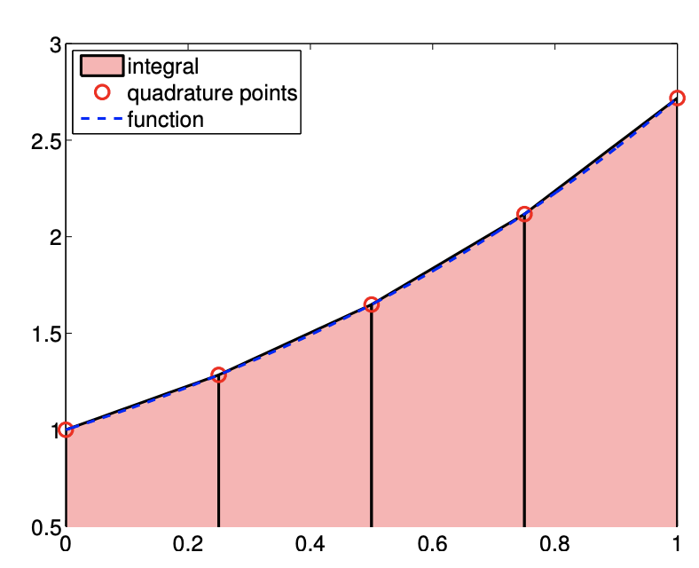
The last integration rule considered is the trapezoidal rule, which is based on the linear interpolant formed by using the interpolation points \(\bar{x}^{1}=x_{i}\) and \(\bar{x}^{2}=x_{i+1}\) on each segment \(S_{i}=\left[x_{i}, x_{i+1}\right]\). The integration formula is given by \[\begin{aligned} I_{h} &=\sum_{i=1}^{N-1} \int_{S_{i}}(\mathcal{I} f)(x) d x=\sum_{i=1}^{N-1} \int_{S_{i}}\left[f\left(x_{i}\right)+\left(\frac{f\left(x_{i+1}\right)-f\left(x_{i}\right)}{h}\right)\left(x-x_{i}\right)\right] \\ &=\sum_{i=1}^{N-1}\left[f\left(x_{i}\right) h+\frac{1}{2}\left(f\left(x_{i+1}\right)-f\left(x_{i}\right)\right) h\right] \\ &=\sum_{i=1}^{N-1} \frac{1}{2} h\left(f\left(x_{i}\right)+f\left(x_{i+1}\right)\right) . \end{aligned}\] As the global function evaluation points are related to the segmentation points by \(\tilde{x}_{i}=x_{i}, i=\) \(1, \ldots, N\), the quadrature rule can also be expressed as \[I_{h}=\sum_{i=1}^{N-1} \frac{1}{2} h\left(f\left(\tilde{x}_{i}\right)+f\left(\tilde{x}_{i+1}\right)\right),\] Rearranging the equation, we can write the integration rule as \[I_{h}=\sum_{i=1}^{N-1} \frac{1}{2} h\left(f\left(\tilde{x}_{i}\right)+f\left(\tilde{x}_{i+1}\right)\right)=\frac{1}{2} h f\left(\tilde{x}_{1}\right)+\sum_{i=2}^{N-1}\left[h f\left(\tilde{x}_{i}\right)\right]+\frac{1}{2} h f\left(\tilde{x}_{N}\right) .\] Note that this quadrature rule assigns a different quadrature weight to the quadrature points on the domain boundary from the points in the interior of the domain. The integration rule is illustrated in Figure 7.5(a).

Using the general integration formula, Eq. (7.7), we obtain the error bound \[\left|I-I_{h}\right| \leq(b-a) e_{\max }=(b-a) \frac{h^{2}}{8} \max _{x \in[a, b]}\left|f^{\prime \prime}(x)\right| .\]

(a) integral

(b) error

Figure 7.5: Trapezoidal rule.

This bound can be tightened by a constant factor, yielding \[\left|I-I_{h}\right| \leq(b-a) e_{\max }=(b-a) \frac{h^{2}}{12} \max _{x \in[a, b]}\left|f^{\prime \prime}(x)\right|\] which is sharp. The error bound shows that the scheme is second-order accurate.

Proof

To prove the sharp bound of the integration error, recall the following intermediate result from the proof of the linear interpolation error, Eq. (2.3), \[f(x)-(\mathcal{I} f)(x)=\frac{1}{2} f^{\prime \prime}\left(\xi_{i}\right)\left(x-x_{i}\right)\left(x-x_{i+1}\right)\] for some \(\xi_{i} \in\left[x_{i}, x_{i+1}\right]\). Integrating the expression over the segment \(S_{i}\), we obtain the local error representation \[\begin{aligned} I^{n}-I_{h}^{n} &=\int_{x_{i}}^{x_{i+1}} f(x)-(\mathcal{I} f)(x) d x=\int_{x_{i}}^{x_{i+1}} \frac{1}{2} f^{\prime \prime}\left(\xi_{i}\right)\left(x-x_{i}\right)\left(x-x_{i+1}\right) d x \\ & \leq \int_{x_{i}}^{x_{i+1}} \frac{1}{2}\left|f^{\prime \prime}\left(\xi_{i}\right)\left(x-x_{i}\right)\left(x-x_{i+1}\right)\right| d x \leq\left(\int_{x_{i}}^{x_{i+1}} \frac{1}{2}\left|\left(x-x_{i}\right)\left(x-x_{i+1}\right)\right| d x\right)_{\xi \in\left[x_{i}, x_{i+1}\right]}\left|f^{\prime \prime}(\xi)\right| \\ &=\frac{1}{12}\left(x_{i+1}-x_{i}\right)^{3} \max _{\xi \in\left[x_{i}, x_{i+1}\right]}\left|f^{\prime \prime}(\xi)\right|=\frac{1}{12} h^{3} \max _{\xi \in\left[x_{i}, x_{i+1}\right]}\left|f^{\prime \prime}(\xi)\right| \end{aligned}\] Summing the local errors, we obtain the global error bound \[\left|I-I_{h}\right|=\left|\sum_{i=1}^{N} \frac{1}{12} h^{3} \max _{\xi_{i} \in\left[x_{i}, x_{i+1}\right]}\right| f^{\prime \prime}\left(\xi_{i}\right)\left|\leq \frac{1}{12}(b-a) h^{2} \max _{x \in[a, b]}\right| f^{\prime \prime}(x) \mid\]

(a) integral

(b) error

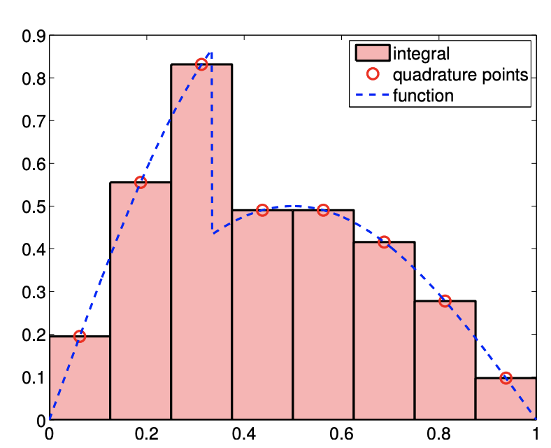
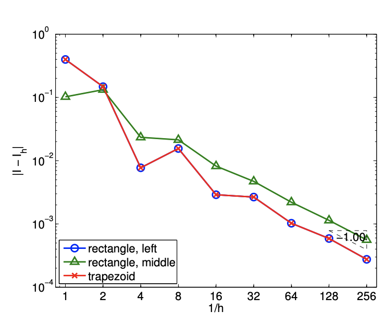
Figure 7.6: Integration of a non-smooth function.

Before concluding this section, let us make a few remarks regarding integration of a non-smooth function. For interpolation, we saw that the maximum error can be no better than \(h^{r}\), where \(r\) is the highest order derivative that is defined everywhere in the domain. For integration, the regularity requirement is less stringent. To see this, let us again consider our discontinuous function \[f(x)=\left\{\begin{array}{ll} \sin (\pi x), & x \leq \frac{1}{3} \\ \frac{1}{2} \sin (\pi x), & x>\frac{1}{3} \end{array} .\right.\] The result of applying the midpoint integration rule with eight intervals is shown in Figure 7.6(a). Intuitively, we can see that the area covered by the approximation approaches that of the true area even in the presence of the discontinuity as \(h \rightarrow 0\). Figure \(7.6(\mathrm{~b})\) confirms that this indeed is the case. All schemes considered converge at the rate of \(h^{1}\). The convergence rate for the midpoint and trapezoidal rules are reduced to \(h^{1}\) from \(h^{2}\). Formally, we can show that the integration schemes converge at the rate of \(\min (k, r+1)\), where \(k\) is the order of accuracy of the integration scheme for a smooth problem, and \(r\) is the highest-order derivative of \(f\) that is defined everywhere in the domain. In terms of accuracy, integration smooths and thus helps, whereas differentiation amplifies variations and hence hurts.