7.2: Integration of Bivariate Functions

Having interpolated bivariate functions, we now consider integration of bivariate functions. We wish to approximate \[I=\iint_{D} f(x, y) d x d y .\] Following the approach used to integrate univariate functions, we replace the function \(f\) by its interpolant and integrate the interpolant exactly.

(a) integral

(b) error

Figure 7.7: Midpoint rule.

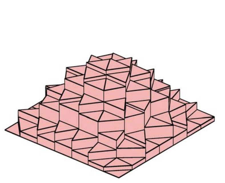
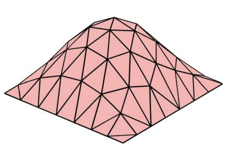
We triangulate the domain \(D\) as shown in Figure \(2.15\) for constructing interpolants. Then, we approximate the integral as the sum of the contributions from the triangles, \(\left\{R_{i}\right\}_{i=1}^{N}\), i.e. \[I=\sum_{i=1}^{N} \iint_{R_{i}} f(x, y) d x d y \approx \sum_{i=1}^{N} \iint_{R_{i}}(\mathcal{I} f)(x, y) d x d y \equiv I_{h}\] We now consider two examples of integration rules.

Example 7.2.1 midpoint rule

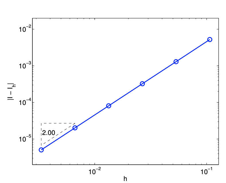
The first rule is the midpoint rule based on the piecewise-constant, midpoint interpolant. Recall, the interpolant over \(R_{i}\) is defined by the function value at its centroid, \[(\mathcal{I} f)(\boldsymbol{x})=f\left(\tilde{\boldsymbol{x}}_{i}\right)=f\left(\boldsymbol{x}_{i}^{c}\right), \quad \forall \boldsymbol{x} \in R^{n}\] where the centroid is given by averaging the vertex coordinates, \[\tilde{\boldsymbol{x}}_{i}=\boldsymbol{x}_{i}^{c}=\frac{1}{3} \sum_{i=1}^{3} \boldsymbol{x}_{i}\] The integral is approximated by \[I_{h}=\sum_{i=1}^{N} \iint_{R_{i}}(\mathcal{I} f)(x, y) d x d y=\sum_{i=1}^{N} \iint_{R_{i}} f\left(\tilde{x}_{i}, \tilde{y}_{i}\right) d x d y=\sum_{i=1}^{N} A_{i} f\left(\tilde{x}_{i}, \tilde{y}_{i}\right)\] where we have used the fact \[\iint_{R_{i}} d x d y=A_{i}\] with \(A_{i}\) denoting the area of triangle \(R_{i}\). The integration process is shown pictorially in Figure \(7.7(\mathrm{a})\). Note that this is a generalization of the midpoint rule to two dimensions.

The error in the integration is bounded by \[e \leq C h^{2}\left\|\nabla^{2} f\right\|_{F}\]

(a) integral

(b) error

Figure 7.8: Trapezoidal rule.

Thus, the integration rule is second-order accurate. An example of error convergence is shown Figure 7.7(b), where the triangles are uniformly divided to produce a better approximation of the integral. The convergence plot confirms the second-order convergence of the scheme.

Similar to the midpoint rule in one dimension, the midpoint rule on a triangle also belongs in the family of Gauss quadratures. The quadrature points and weights are chosen optimally to achieve as high-order convergence as possible.

Example 7.2.2 trapezoidal rule

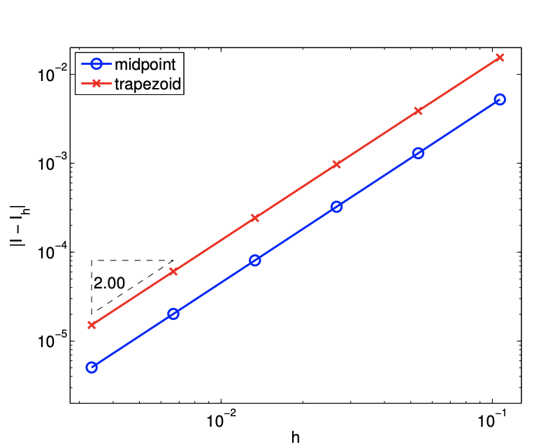
The trapezoidal-integration rule is based on the piecewise-linear interpolant. Because the integral of a linear function defined on a triangular patch is equal to the average of the function values at its vertices times the area of the triangle, the integral simplifies to \[I_{h}=\sum_{i=1}^{N}\left[\frac{1}{3} A_{i} \sum_{m=1}^{3} f\left(\bar{x}_{i}^{m}\right)\right]\] where \(\left\{\overline{\boldsymbol{x}}_{i}^{1}, \overline{\boldsymbol{x}}_{i}^{2}, \overline{\boldsymbol{x}}_{i}^{3}\right\}\) are the vertices of the triangle \(R_{i}\). The integration process is graphically shown in Figure 7.8(a).

The error in the integration is bounded by \[e \leq C h^{2}\left\|\nabla^{2} f\right\|_{F}\] The integration rule is second-order accurate, as confirmed by the convergence plot shown in Figure \(7.8(\mathrm{~b})\).

The integration rules extend to higher dimensions in principle by using interpolation rules for higher dimensions. However, the number of integration points increases as \((1 / h)^{d}\), where \(d\) is the physical dimension. The number of points increases exponentially in \(d\), and this is called the curse of dimensionality. An alternative is to use a integration process based on random numbers, which is discussed in the next unit.