9.3: Binomial Distribution

In the previous section, we saw random vectors consisting of two random variables, \(X\) and \(Y\). Let us generalize the concept and introduce a random vector consisting of \(n\) components \[\left(X_{1}, X_{2}, \ldots, X_{n}\right),\] where each \(X_{i}\) is a random variable. In particular, we are interested in the case where each \(X_{i}\) is a Bernoulli random variable with the probability of success of \(\theta\). Moreover, we assume that \(X_{i}\), \(i=1, \ldots, n\), are independent. Because the random variables are independent and each variable has the same distribution, they are said to be independent and identically distributed or i.i.d. for short. In other words, if a set of random variables \(X_{1}, \ldots, X_{n}\) is i.i.d., then \[f_{X_{1}, X_{2}, \ldots, X_{n}}\left(x_{1}, x_{2}, \ldots, x_{n}\right)=f_{X}\left(x_{1}\right) \cdot f_{X}\left(x_{2}\right) \cdots f_{X}\left(x_{n}\right),\] where \(f_{X}\) is the common probability density for \(X_{1}, \ldots, X_{n}\). This concept plays an important role in statistical inference and allows us to, for example, make a probabilistic statement about behaviors of random experiments based on observations.

Now let us transform the i.i.d. random vector \(\left(X_{1}, \ldots, X_{n}\right)\) of Bernoulli random variables to a random variable \(Z\) by summing its components, i.e. \[Z_{n}=\sum_{i=1}^{n} X_{i} .\] (More precisely we should write \(Z_{n, \theta}\) since \(Z\) depends on both \(n\) and \(\theta\).) Note \(Z_{n}\) is a function of \(\left(X_{1}, X_{2}, \ldots, X_{n}\right)\), and in fact a simple function - the sum. Because \(X_{i}, i=1, \ldots, n\), are random variables, their sum is also a random variable. In fact, this sum of Bernoulli random variable is called a binomial random variable. It is denoted by \(Z_{n} \sim \mathcal{B}(n, \theta)\) (shorthand for \(f_{Z_{n, \theta}}(z)=\) \(\left.f^{\text {binomial }}(z ; n, \theta)\right)\), where \(n\) is the number of Bernoulli events and \(\theta\) is the probability of success of each event. Let us consider a few examples of binomial distributions.

Example 9.3.1 total number of heads in flipping two fair coins

Let us first revisit the case of flipping two fair coins. The random vector considered in this case is \[\left(X_{1}, X_{2}\right) \text {, }\] where \(X_{1}\) and \(X_{2}\) are independent Bernoulli random variables associated with the first and second flip, respectively. As in the previous coin flip cases, we associate 1 with heads and 0 with tails. There are four possible outcome of these flips, \[(0,0), \quad(0,1), \quad(1,0), \quad \text { and }(1,1) \text {. }\] From the two flips, we can construct the binomial distribution \(Z_{2} \sim \mathcal{B}(2, \theta=1 / 2)\), corresponding to the total number of heads that results from flipping two fair coins. The binomial random variable is defined as \[Z_{2}=X_{1}+X_{2} .\] Counting the number of heads associated with all possible outcomes of the coin flip, the binomial random variable takes on the following value:

First flip	0	0	1	1
Second flip	0	1	0	1
\(Z_{2}\)	0	1	1	2

Because the coin flips are independent and each coin flip has the probability density of \(f_{X_{i}}(x)=1 / 2\), \(x=0,1\), their joint distribution is \[f_{X_{1}, X_{2}}\left(x_{1}, x_{2}\right)=f_{X_{1}}\left(x_{1}\right) \cdot f_{X_{2}}\left(x_{2}\right)=\frac{1}{2} \cdot \frac{1}{2}=\frac{1}{4}, \quad\left(x_{1}, x_{2}\right) \in\{(0,0),(0,1),(1,0),(1,1)\} .\] In words, each of the four possible events are equally likely. Of these four equally likely events, \(Z_{2} \sim \mathcal{B}(2,1 / 2)\) takes on the value of 0 in one event, 1 in two events, and 2 in one event. Thus, the behavior of the binomial random variable \(Z_{2}\) can be concisely stated as \[Z_{2}= \begin{cases}0, & \text { with probability } 1 / 4 \\ 1, & \text { with probability } 1 / 2(=2 / 4) \\ 2, & \text { with probability } 1 / 4\end{cases}\] Note this example is very similar to Example 9.1.4: \(Z_{2}\), the sum of \(X_{1}\) and \(X_{2}\), is our \(g(X)\); we assign probabilities by invoking the mutually exclusive property, OR (union), and summation. Note that the mode, the value that \(Z_{2}\) is most likely to take, is 1 for this case. The probability mass function of \(Z_{2}\) is given by \[f_{Z_{2}}(x)= \begin{cases}1 / 4, & x=0 \\ 1 / 2, & x=1 \\ 1 / 4, & x=2\end{cases}\]

Example 9.3.2 total number of heads in flipping three fair coins

Let us know extend the previous example to the case of flipping a fair coin three times. In this case, the random vector considered has three components, \[\left(X_{1}, X_{2}, X_{3}\right) \text {, }\] with each \(X_{1}\) being a Bernoulli random variable with the probability of success of \(1 / 2\). From the three flips, we can construct the binomial distribution \(Z_{3} \sim \mathcal{B}(3,1 / 2)\) with \[Z_{3}=X_{1}+X_{2}+X_{3} .\] The all possible outcomes of the random vector and the associated outcomes of the binomial distribution are:

First flip	0	1	0	0	1	0	1	1
Second flip	0	0	1	0	1	1	0	1
Third flip	0	0	0	1	0	1	1	1
\(Z_{3}\)	0	1	1	1	2	2	2	3

Because the Bernoulli random variables are independent, their joint distribution is \[f_{X_{1}, X_{2}, X_{3}}\left(x_{1}, x_{2}, x_{3}\right)=f_{X_{1}}\left(x_{1}\right) \cdot f_{X_{2}}\left(x_{2}\right) \cdot f_{X_{3}}\left(x_{3}\right)=\frac{1}{2} \cdot \frac{1}{2} \cdot \frac{1}{2}=\frac{1}{8} .\] In other words, each of the eight events is equally likely. Of the eight equally likely events, \(Z_{3}\) takes on the value of 0 in one event, 1 in three events, 2 in three events, and 3 in one event. The behavior of the binomial variable \(Z_{3}\) is summarized by \[Z_{3}= \begin{cases}0, & \text { with probability } 1 / 8 \\ 1, & \text { with probability } 3 / 8 \\ 2, & \text { with probability } 3 / 8 \\ 3, & \text { with probability } 1 / 8\end{cases}\] The probability mass function (for \(\theta=1 / 2\) ) is thus given by \[f_{Z_{3}}(x)= \begin{cases}1 / 8, & x=0 \\ 3 / 8, & x=1 \\ 3 / 8, & x=2 \\ 1 / 8, & x=3 .\end{cases}\]

Example 9.3.3 total number of heads in flipping four fair coins

We can repeat the procedure for four flips of fair coins \((n=4\) and \(\theta=1 / 2)\). In this case, we consider the sum of the entries of a random vector consisting of four Bernoulli random variables, \(\left(X_{1}, X_{2}, X_{3}, X_{4}\right)\). The behavior of \(Z_{4}=\mathcal{B}(4,1 / 2)\) is summarized by \[Z_{4}= \begin{cases}0, & \text { with probability } 1 / 16 \\ 1, & \text { with probability } 1 / 4 \\ 2, & \text { with probability } 3 / 8 \\ 3, & \text { with probability } 1 / 4 \\ 4, & \text { with probability } 1 / 16\end{cases}\] Note that \(Z_{4}\) is much more likely to take on the value of 2 than 0 , because there are many equallylikely events that leads to \(Z_{4}=2\), whereas there is only one event that leads to \(Z_{4}=0\). In general, as the number of flips increase, the deviation of \(Z_{n} \sim \mathcal{B}(n, \theta)\) from \(n \theta\) becomes increasingly unlikely.

Figure \(9.9\) illustrates the values taken by binomial random variables for \(n=2\) and \(n=4\), both with \(\theta=\overline{1 / 2}\). The histogram confirms that the distribution is more likely to take on the values near the mean because there are more sequences of the coin flips that realizes these values. We also note that the values become more concentrated near the mean, \(n \theta\), relative to the range of the values it can take, \([0, n]\), as \(n\) increases. This is reflected in the decrease in the standard deviation relative to the width of the range of the values \(Z_{n}\) can take.

In general, a binomial random variable \(Z_{n} \sim \mathcal{B}(n, \theta)\) behaves as \[Z_{n}=k, \quad \text { with probability }\left(\begin{array}{c} n \\ k \end{array}\right) \theta^{k}(1-\theta)^{n-k},\] where \(k=1, \ldots, n\). Recall that \(\left(\begin{array}{l}n \\ k\end{array}\right)\) is the binomial coefficient, read " \(n\) choose \(k\) : the number of ways of picking \(k\) unordered outcomes from \(n\) possibilities. The value can be evaluated as \[\left(\begin{array}{l} n \\ k \end{array}\right) \equiv \frac{n !}{(n-k) ! k !},\]

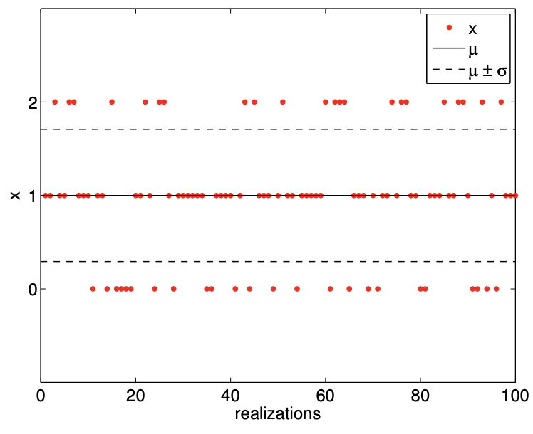
(a) realization, \(n=2, \theta=1 / 2\)

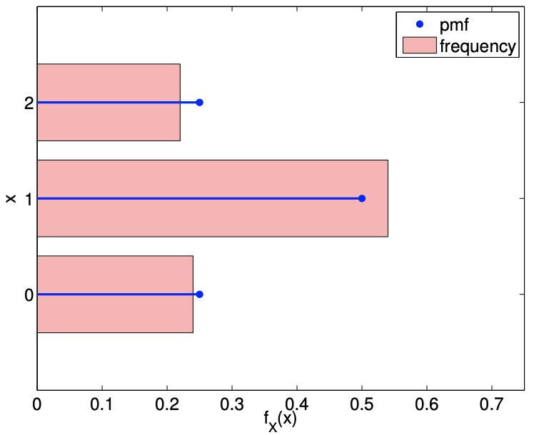
(b) pmf, \(n=2, \theta=1 / 2\)

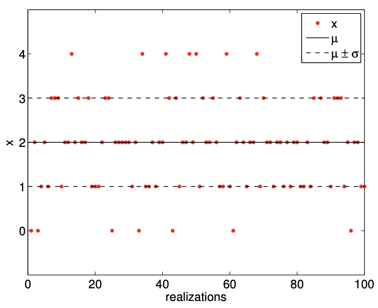
(c) realization, \(n=4, \theta=1 / 2\)

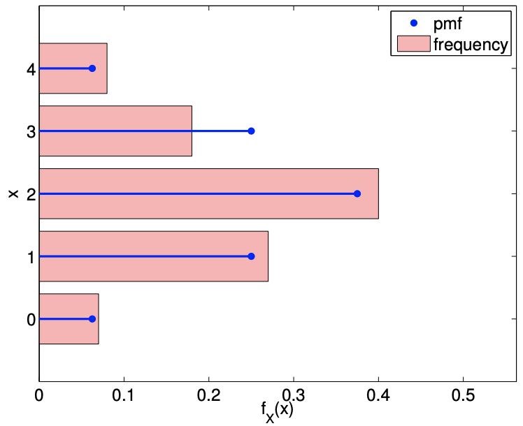
(d) pmf, \(n=4, \theta=1 / 2\)

Figure 9.9: Illustration of the values taken by binomial random variables.

where ! denotes the factorial.

We can readily derive the formula for \(\mathcal{B}(n, \theta)\). We think of \(n\) tosses as a binary number with \(n\) bits, and we ask how many ways \(k\) ones can appear. We can place the first one in \(n\) different places, the second one in \(n-1\) different places, ..., which yields \(n ! /(n-k)\) ! possibilities. But since we are just counting the number of ones, the order of appearance does not matter, and we must divide \(n ! /(n-k) !\) by the number of different orders in which we can construct the same pattern of \(k\) ones - the first one can appear in \(k\) places, the second one in \(k-1\) places, ..., which yields \(k\) !. Thus there are " \(n\) choose \(k\) " ways to obtain \(k\) ones in a binary number of length \(n\), or equivalently " \(n\) choose \(k\) " different binary numbers with \(k\) ones. Next, by independence, each pattern of \(k\) ones (and hence \(n-k\) zeros) has probability \(\theta^{k}(1-\theta)^{n-k}\). Finally, by the mutually exclusive property, the probability that \(Z_{n}=k\) is simply the number of patterns with \(k\) ones multiplied by the probability that each such pattern occurs (note the probability is the same for each such pattern).

The mean and variance of a binomial distribution is given by \[E\left[Z_{n}\right]=n \theta \text { and } \operatorname{Var}\left[Z_{n}\right]=n \theta(1-\theta) .\]

Proof

The proof for the mean follows from the linearity of expectation, i.e. \[E\left[Z_{n}\right]=E\left[\sum_{i=1}^{n} X_{i}\right]=\sum_{i=1}^{n} E\left[X_{i}\right]=\sum_{i=1}^{n} \theta=n \theta .\] Note we can readily prove that the expectation of the sum is the sum of the expectations. We consider the \(n\)-dimensional sum over the joint mass function of the \(X_{i}\) weighted - per the definition of expectation - by the sum of the \(X_{i}, i=1, \ldots, n\). Then, for any given \(X_{i}\), we factorize the joint mass function: \(n-1\) of the sums then return unity, while the last sum gives the expectation of \(X_{i}\). The proof for variance relies on the pairwise independence of the random variables \[\begin{aligned} \operatorname{Var}\left[Z_{n}\right] &\left.=E\left[\left(Z_{n}-E\left[Z_{n}\right]\right)^{2}\right]=E\left[\left\{\left(\sum_{i=1}^{n} X_{i}\right)-n \theta\right\}^{2}\right]=E\left[\left\{\sum_{i=1}^{n}\left(X_{i}-\theta\right)\right\}^{2}\right]\right] \\ &=E\left[\sum_{i=1}^{n}\left(X_{i}-\theta\right)^{2}+\sum_{i=1}^{n} \sum_{\substack{j=1 \\ j \neq i}}^{n}\left(X_{i}-\theta\right)\left(X_{j}-\theta\right)\right] \\ &=\sum_{i=1}^{n} E\left[\left(X_{i}-\theta\right)^{2}\right]+\sum_{\substack{i=1}}^{n} \sum_{\substack{j=1 \\ j \neq i}}^{n} E\left[\left(X_{i}=\theta\right)\left(X_{j}-\theta\right)\right] \\ &=\sum_{i=1}^{n} \operatorname{Var}\left[X_{i}\right]=\sum_{i=1}^{n} \theta(1-\theta)=n \theta(1-\theta) \end{aligned}\] The cross terms cancel because coin flips are independent.

Note that the variance scales with \(n\), or, equivalently, the standard deviation scales with \(\sqrt{n}\). This turns out to be the key to Monte Carlo methods - numerical methods based on random variables - which is the focus of the later chapters of this unit.

Let us get some insight to how the general formula works by applying it to the binomial distribution associated with flipping coins three times.

Example 9.3.4 applying the general formula to coin flips

Let us revisit \(Z_{3}=\mathcal{B}(3,1 / 2)\) associated with the number of heads in flipping three coins. The probability that \(Z_{3}=0\) is, by substituting \(n=3, k=0\), and \(\theta=1 / 2\), \[f_{Z_{3}}(0)=\left(\begin{array}{c} n \\ k \end{array}\right) \theta^{k}(1-\theta)^{n-k}=\left(\begin{array}{c} 3 \\ 0 \end{array}\right)\left(\frac{1}{2}\right)^{0}\left(1-\frac{1}{2}\right)^{3-0}=\frac{3 !}{0 !(3-0) !}\left(\frac{1}{2}\right)^{3}=\frac{1}{8},\] which is consistent with the probability we obtained previously. Let us consider another case: the probability of \(Z_{3}=2\) is \[f_{Z_{3}}(2)=\left(\begin{array}{c} n \\ k \end{array}\right) \theta^{k}(1-\theta)^{n-k}=\left(\begin{array}{l} 3 \\ 2 \end{array}\right)\left(\frac{1}{2}\right)^{2}\left(1-\frac{1}{2}\right)^{3-2}=\frac{3 !}{2 !(3-2) !}\left(\frac{1}{2}\right)^{3}=\frac{3}{8} .\] Note that the \(\theta^{k}(1-\theta)^{n-k}\) is the probability that the random vector of Bernoulli variables \[\left(X_{1}, X_{2}, \ldots, X_{n}\right),\] realizes \(X_{1}=X_{2}=\ldots=X_{k}=1\) and \(X_{k+1}=\ldots=X_{n}=0\), and hence \(Z_{n}=k\). Then, we multiply the probability with the number of different ways that we can realize the sum \(Z_{n}=k\), which is equal to the number of different way of rearranging the random vector. Here, we are using the fact that the random variables are identically distributed. In the special case of (fair) coin flips, \(\theta^{k}(1-\theta)^{n-k}=(1 / 2)^{k}(1-1 / 2)^{n-k}=(1 / 2)^{n}\), because each random vector is equally likely.