9.4: Continuous Random Variables

Probability Density Function; Cumulative Distribution Function

Let \(X\) be a random variable that takes on any real value in (say) an interval, \[X \in[a, b] .\] The probability density function (pdf) is a function over \([a, b], f_{X}(x)\), such that \[\begin{aligned} f_{X}(x) & \geq 0, \quad \forall x \in[a, b], \\ \int_{a}^{b} f_{X}(x) d x &=1 . \end{aligned}\] Note that the condition that the probability mass function sums to unity is replaced by an integral condition for the continuous variable. The probability that \(X\) take on a value over an infinitesimal interval of length \(d x\) is \[P(x \leq X \leq x+d x)=f_{X}(x) d x,\] or, over a finite subinterval \(\left[a^{\prime}, b^{\prime}\right] \subset[a, b]\), \[P\left(a^{\prime} \leq X \leq b^{\prime}\right)=\int_{a^{\prime}}^{b^{\prime}} f_{X}(x) d x .\] In other words, the probability that \(X\) takes on the value between \(a^{\prime}\) and \(b^{\prime}\) is the integral of the probability density function \(f_{X}\) over \(\left[a^{\prime}, b^{\prime}\right]\).

A particular instance of this is a cumulative distribution function (cdf), \(F_{X}(x)\), which describes the probability that \(X\) will take on a value less than \(x\), i.e. \[F_{X}(x)=\int_{a}^{x} f_{X}(x) d x .\] (We can also replace \(a\) with \(-\infty\) if we define \(f_{X}(x)=0\) for \(-\infty<x<a\).) Note that any cdf satisfies the conditions \[F_{X}(a)=\int_{a}^{a} f_{X}(x) d x=0 \quad \text { and } \quad F_{X}(b)=\int_{a}^{b} f_{X}(x) d x=1\] Furthermore, it easily follows from the definition that \[P\left(a^{\prime} \leq X \leq b^{\prime}\right)=F_{X}\left(b^{\prime}\right)-F_{X}\left(a^{\prime}\right) .\] That is, we can compute the probability of \(X\) taking on a value in \(\left[a^{\prime}, b^{\prime}\right]\) by taking the difference of the cdf evaluated at the two end points.

Let us introduce a few notions useful for characterizing a pdf, and thus the behavior of the random variable. The mean, \(\mu\), or the expected value, \(E[X]\), of the random variable \(X\) is \[\mu=E[X]=\int_{a}^{b} f(x) x d x .\] The variance, \(\operatorname{Var}(X)\), is a measure of the spread of the values that \(X\) takes about its mean and is defined by \[\operatorname{Var}(X)=E\left[(X-\mu)^{2}\right]=\int_{a}^{b}(x-\mu)^{2} f(x) d x .\] The variance can also be expressed as \[\begin{aligned} \operatorname{Var}(X) &=E\left[(X-\mu)^{2}\right]=\int_{a}^{b}(x-\mu)^{2} f(x) d x \\ &=\int_{a}^{b} x^{2} f(x) d x-2 \mu \underbrace{\int_{a}^{b} x f(x) d x}_{\mu}+\mu^{2} \int_{a}^{b} f(x) d x \\ &=E\left[X^{2}\right]-\mu^{2} . \end{aligned}\] The \(\alpha\)-th quantile of a random variable \(X\) is denoted by \(\tilde{z}_{\alpha}\) and satisfies \[F_{X}\left(\tilde{z}_{\alpha}\right)=\alpha .\] In other words, the quantile \(\tilde{z}_{\alpha}\) partitions the interval \([a, b]\) such that the probability of \(X\) taking on a value in \(\left[a, \tilde{z}_{\alpha}\right]\) is \(\alpha\) (and conversely \(\left.P\left(\tilde{z}_{\alpha} \leq X \leq b\right)=1-\alpha\right)\). The \(\alpha=1 / 2\) quantile is the median.

Let us consider a few examples of continuous random variables.

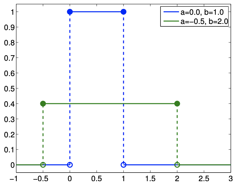
(a) probability density function

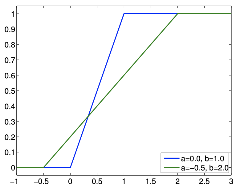
(b) cumulative density function

Figure 9.10: Uniform distributions

Example 9.4.1 Uniform distribution

Let \(X\) be a uniform random variable. Then, \(X\) is characterized by a constant pdf, \[f_{X}(x)=f^{\text {uniform }}(x ; a, b) \equiv \frac{1}{b-a}\] Note that the pdf satisfies the constraint \[\int_{a}^{b} f_{X}(x) d x=\int_{a}^{b} f^{\text {uniform }}(x ; a, b) d x=\int_{a}^{b} \frac{1}{b-a} d x=1\] Furthermore, the probability that the random variable takes on a value in the subinterval \(\left[a^{\prime}, b^{\prime}\right] \in\) \([a, b]\) is \[P\left(a^{\prime} \leq X \leq b^{\prime}\right)=\int_{a^{\prime}}^{b^{\prime}} f_{X}(x) d x=\int_{a^{\prime}}^{b^{\prime}} f^{\text {uniform }}(x ; a, b) d x=\int_{a^{\prime}}^{b^{\prime}} \frac{1}{b-a} d x=\frac{b^{\prime}-a^{\prime}}{b-a}\] In other words, the probability that \(X \in\left[a^{\prime}, b^{\prime}\right]\) is proportional to the relative length of the interval as the density is equally distributed. The distribution is compactly denoted as \(\mathcal{U}(a, b)\) and we write \(X \sim \mathcal{U}(a, b)\). A straightforward integration of the pdf shows that the cumulative distribution function of \(X \sim \mathcal{U}(a, b)\) is \[F_{X}(x)=F^{\text {uniform }}(x ; a, b) \equiv \frac{x-a}{b-a}\] The pdf and cdf for a few uniform distributions are shown in Figure \(9.10\).

An example of the values taken by a uniform random variable \(\mathcal{U}(0,1)\) is shown in Figure \(9.11(\) a) . By construction, the range of values that the variable takes is limited to between \(a=0\) and \(b=1\). As expected, there is no obvious concentration of the values within the range \([a, b]\). Figure \(9.11(b)\) shows a histrogram that summarizes the frequency of the event that \(X\) resides in bins \(\left[x_{i}, x_{i}+\delta x\right]\), \(i=1, \ldots, n_{\text {bin. }}\). The relative frequency of occurrence is normalized by \(\delta x\) to be consistent with the definition of the probability density function. In particular, the integral of the region filled by the histogram is unity. While there is some spread in the frequencies of occurrences due to

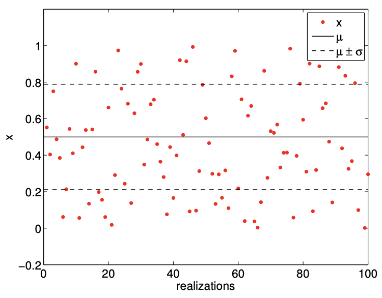
(a) realization

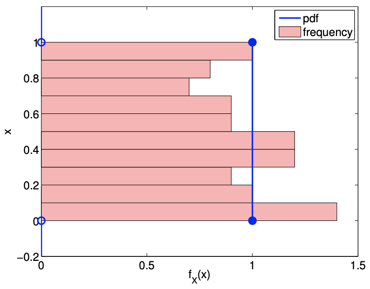
(b) probability density

Figure 9.11: Illustration of the values taken by an uniform random variable \((a=0, b=1)\).

the relatively small sample size, the histogram resembles the probability density function. This is consistent with the frequentist interpretation of probability.

The mean of the uniform distribution is given by \[E[X]=\int_{a}^{b} x f_{X}(x) d x=\int_{a}^{b} x \frac{1}{b-a} d x=\frac{1}{2}(a+b)\] This agrees with our intuition, because if \(X\) is to take on a value between \(a\) and \(b\) with equal probability, then the mean would be the midpoint of the interval. The variance of the uniform distribution is \[\begin{aligned} \operatorname{Var}(X) &=E\left[X^{2}\right]-(E[X])^{2}=\int_{a}^{b} x^{2} f_{X}(x) d x-\left(\frac{1}{2}(a+b)\right)^{2} \\ &=\int_{a}^{b} \frac{x^{2}}{b-a} d x-\left(\frac{1}{2}(a+b)\right)^{2}=\frac{1}{12}(b-a)^{2} \end{aligned}\]

Example 9.4.2 Normal distribution

Let \(X\) be a normal random variable. Then the probability density function of \(X\) is of the form \[f_{X}(x)=f^{\text {normal }}\left(x ; \mu, \sigma^{2}\right) \equiv \frac{1}{\sqrt{2 \pi} \sigma} \exp \left(-\frac{(x-\mu)^{2}}{2 \sigma^{2}}\right)\] The pdf is parametrized by two variables, the mean \(\mu\) and the variance \(\sigma^{2}\). (More precisely we would thus write \(X_{\left.\mu, \sigma^{2} .\right)}\) Note that the density is non-zero over the entire real axis and thus in principle \(X\) can take on any value. The normal distribution is concisely denoted by \(X \sim \mathcal{N}\left(\mu, \sigma^{2}\right)\). The cumulative distribution function of a normal distribution takes the form \[F_{X}(x)=F^{\text {normal }}\left(x ; \mu, \sigma^{2}\right) \equiv \frac{1}{2}\left[1+\operatorname{erf}\left(\frac{x-\mu}{\sqrt{2} \sigma}\right)\right]\]

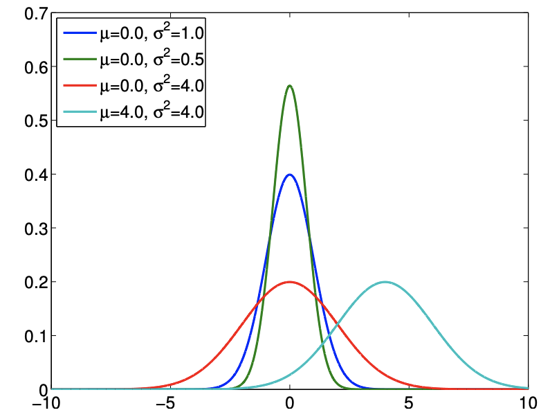
(a) probability density function

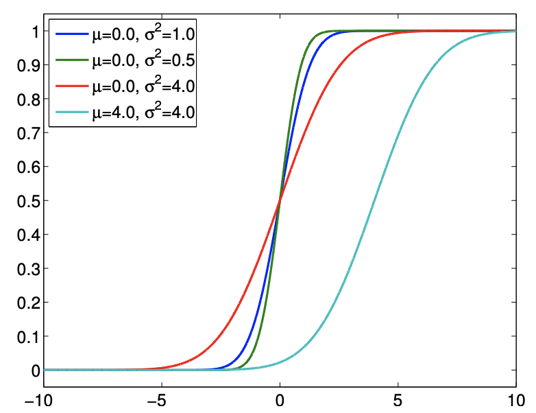
(b) cumulative density function

Figure 9.12: Normal distributions

where erf is the error function, given by \[\operatorname{erf}(x)=\frac{2}{\pi} \int_{0}^{x} e^{-z^{2}} d z\] We note that it is customary to denote the cdf for the standard normal distribution (i.e. \(\mu=0\), \(\sigma^{2}=1\) ) by \(\Phi\), i.e. \[\Phi(x)=F^{\text {normal }}\left(x ; \mu=0, \sigma^{2}=1\right)\] We will see many use of this cdf in the subsequent sections. The pdf and cdf for a few normal distributions are shown in Figure \(9.12\).

An example of the values taken by a normal random variable is shown in Figure \(9.13\). As already noted, \(X\) can in principle take on any real value; however, in practice, as the Gaussian function decays quickly away from the mean, the probability of \(X\) taking on a value many standard deviations away from the mean is small. Figure \(9.13\) clearly illustrates that the values taken by \(X\) is clustered near the mean. In particular, we can deduce from the cdf that \(X\) takes on values within \(\sigma, 2 \sigma\), and \(3 \sigma\) of the mean with probability \(68.2 \%, 95.4 \%\), and \(99.7 \%\), respectively. In other words, the probability of \(X\) taking of the value outside of \(\mu \pm 3 \sigma\) is given by \[1-\int_{\mu-3 \sigma}^{\mu+3 \sigma} f^{\text {normal }}\left(x ; \mu, \sigma^{2}\right) d x \equiv 1-\left(F^{\text {normal }}\left(\mu+3 \sigma ; \mu, \sigma^{2}\right)-F^{\text {normal }}\left(\mu-3 \sigma ; \mu, \sigma^{2}\right)\right) \approx 0.003\] We can easily compute a few quantiles based on this information. For example, \[\tilde{z}_{0.841} \approx \mu+\sigma, \quad \tilde{z}_{0.977} \approx \mu+2 \sigma, \quad \text { and } \quad \tilde{z}_{0.9987} \approx \mu+3 \sigma\] It is worth mentioning that \(\tilde{z}_{0.975} \approx \mu+1.96 \sigma\), as we will frequently use this constant in the subsequent sections.

Although we only consider either discrete or continuous random variables in this notes, random variables can be mixed discrete and continuous in general. Mixed discrete-continuous random variables are characterized by the appearance of discontinuities in their cumulative distribution function.

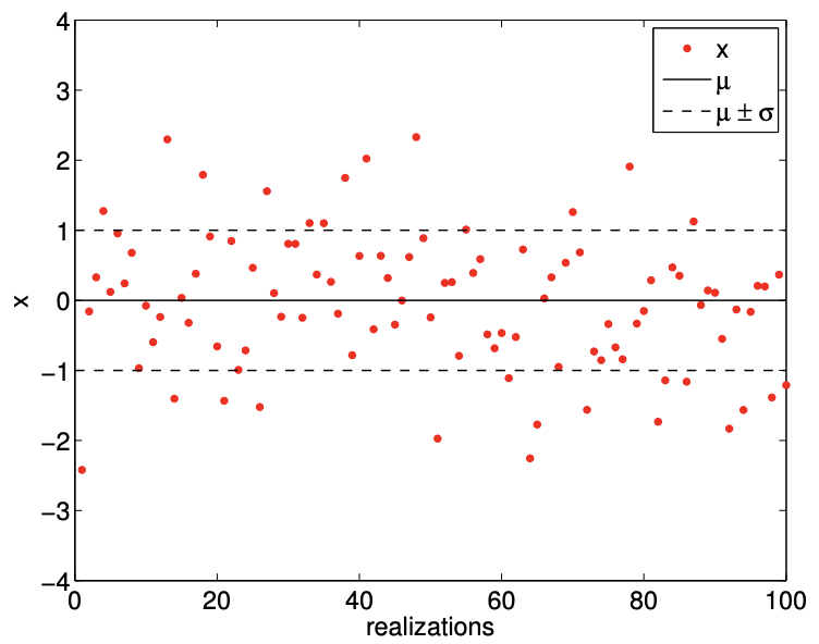
(a) realization

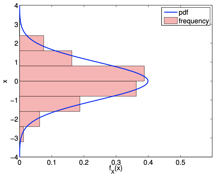
(b) probability density

Figure 9.13: Illustration of the values taken by a normal random variable \((\mu=0, \sigma=1)\).

Transformations of Continuous Random Variables

Just like discrete random variables, continuous random variables can be transformed by a function. The transformation of a random variable \(X\) by a function \(g\) produces another random variable, \(Y\), and we denote this by \[Y=g(X)\] We shall consider here only monotonic functions \(g\).

Recall that we have described the random variable \(X\) by distribution \[P(x \leq X \leq x+d x)=f_{X}(x) d x\] The transformed variable follows \[P(y \leq Y \leq y+d y)=f_{Y}(y) d y\] Substitution of \(y=g(x)\) and \(d y=g^{\prime}(x) d x\) and noting \(g(x)+g^{\prime}(x) d x=g(x+d x)\) results in \[\begin{aligned} f_{Y}(y) d y &=P\left(g(x) \leq g(X) \leq g(x)+g^{\prime}(x) d x\right)=P(g(x) \leq g(X) \leq g(x+d x)) \\ &=P(x \leq X \leq x+d x)=f_{X}(x) d x \end{aligned}\] In other words, \(f_{Y}(y) d y=f_{X}(x) d x\). This is the continuous analog to \(f_{Y}\left(y_{j}\right)=p_{j}=f_{X}\left(x_{j}\right)\) in the discrete case.

We can manipulate the expression to obtain an explicit expression for \(f_{Y}\) in terms of \(f_{X}\) and \(g\). First we note (from monotonicity) that \[y=g(x) \quad \Rightarrow \quad x=g^{-1}(y) \quad \text { and } \quad d x=\frac{d g^{-1}}{d y} d y\] Substitution of the expressions in \(f_{Y}(y) d y=f_{X}(x) d x\) yields \[f_{Y}(y) d y=f_{X}(x) d x=f_{X}\left(g^{-1}(y)\right) \cdot \frac{d g^{-1}}{d y} d y\] or, \[f_{Y}(y)=f_{X}\left(g^{-1}(y)\right) \cdot \frac{d g^{-1}}{d y} .\] Conversely, we can also obtain an explicit expression for \(f_{X}\) in terms of \(f_{Y}\) and \(g\). From \(y=g(x)\) and \(d y=g^{\prime}(x) d x\), we obtain \[f_{X}(x) d x=f_{Y}(y) d y=f_{Y}(g(x)) \cdot g^{\prime}(x) d x \quad \Rightarrow \quad f_{X}(x)=f_{Y}(g(x)) \cdot g^{\prime}(x) .\] We shall consider several applications below.

Assuming \(X\) takes on a value between \(a\) and \(b\), and \(Y\) takes on a value between \(c\) and \(d\), the mean of \(Y\) is \[E[Y]=\int_{c}^{d} y f_{Y}(y) d y=\int_{a}^{b} g(x) f_{X}(x) d x,\] where the second equality follows from \(f_{Y}(y) d y=f_{X}(x) d x\) and \(y=g(x)\).

Example 9.4.3 Standard uniform distribution to a general uniform distribution

As the first example, let us consider the standard uniform distribution \(U \sim \mathcal{U}(0,1)\). We wish to generate a general uniform distribution \(X \sim \mathcal{U}(a, b)\) defined on the interval \([a, b]\). Because a uniform distribution is uniquely determined by the two end points, we simply need to map the end point 0 to \(a\) and the point 1 to \(b\). This is accomplished by the transformation \[g(u)=a+(b-a) u .\] Thus, \(X \sim \mathcal{U}(a, b)\) is obtained by mapping \(U \sim \mathcal{U}(0,1)\) as \[X=a+(b-a) U .\]

Proof

Proof follows directly from the transformation of the probability density function. The probability density function of \(U\) is \[f_{U}(u)=\left\{\begin{array}{ll} 1, & u \in[0,1] \\ 0, & \text { otherwise } \end{array} .\right.\] The inverse of the transformation \(x=g(u)=a+(b-a) u\) is \[g^{-1}(x)=\frac{x-a}{b-a} .\] From the transformation of the probability density function, \(f_{X}\) is \[f_{X}(x)=f_{U}\left(g^{-1}(x)\right) \cdot \frac{d g^{-1}}{d x}=f_{U}\left(\frac{x-a}{b-a}\right) \cdot \frac{1}{b-a} .\] We note that \(f_{U}\) evaluates to 1 if \[0 \leq \frac{x-a}{b-a} \leq 1 \quad \Rightarrow \quad a \leq x \leq b,\] and \(f_{U}\) evaluates to 0 otherwise. Thus, \(f_{X}\) simplifies to \[f_{X}(x)=\left\{\begin{array}{l} \frac{1}{b-a}, \quad x \in[a, b] \\ 0, \quad \text { otherwise } \end{array}\right.\] which is precisely the probability density function of \(\mathcal{U}(a, b)\).

Example 9.4.4 Standard uniform distribution to a discrete distribution

The uniform distribution can also be mapped to a discrete random variable. Consider a discrete random variable \(Y\) takes on three values \((J=3)\), with \[y_{1}=0, \quad y_{2}=2, \quad \text { and } \quad y_{3}=3\] with probability \[f_{Y}(y)= \begin{cases}1 / 2, & y_{1}=0 \\ 1 / 4, & y_{2}=2 \\ 1 / 4, & y_{3}=3\end{cases}\] To generate \(Y\), we can consider a discontinuous function \(g\). To get the desired discrete probability distribution, we subdivide the interval \([0,1]\) into three subintervals of appropriate lengths. In particular, to generate \(Y\), we consider \[g(x)=\left\{\begin{array}{ll} 0, & x \in[0,1 / 2) \\ 2, & x \in[1 / 2,3 / 4) \\ 3, & x \in[3 / 4,1] \end{array} .\right.\] If we consider \(Y=g(U)\), we have \[Y= \begin{cases}0, & U \in[0,1 / 2) \\ 2, & U \in[1 / 2,3 / 4) \\ 3, & U \in[3 / 4,1]\end{cases}\] Because the probability that the standard uniform random variable takes on a value within a subinterval \(\left[a^{\prime}, b^{\prime}\right]\) is equal to \[P\left(a^{\prime} \leq U \leq b^{\prime}\right)=\frac{b^{\prime}-a^{\prime}}{1-0}=b^{\prime}-a^{\prime},\] the probability that \(Y\) takes on 0 is \(1 / 2-0=1 / 2\), on 2 is \(3 / 4-1 / 2=1 / 4\), and on 3 is \(1-3 / 4=1 / 4\). This gives the desired probability distribution of \(Y\).

Example 9.4.5 Standard normal distribution to a general normal distribution

Suppose we have the standard normal distribution \(Z \sim \mathcal{N}(0,1)\) and wish to map it to a general normal distribution \(X \sim \mathcal{N}\left(\mu, \sigma^{2}\right)\) with the mean \(\mu\) and the variance \(\sigma^{2}\). The transformation is given by \[X=\mu+\sigma Z .\] Conversely, we can map any normal distribution to the standard normal distribution by \[Z=\frac{X-\mu}{\sigma}\]

Proof

The probability density function of the standard normal distribution \(Z \sim \mathcal{N}(0,1)\) is \[f_{Z}(z)=\frac{1}{\sqrt{2 \pi}} \exp \left(-\frac{z^{2}}{2}\right) .\] Using the transformation of the probability density and the inverse mapping, \(z(x)=(x-\mu) / \sigma\), we obtain \[f_{X}(x)=f_{Z}(z(x)) \frac{d z}{d x}=f_{Z}\left(\frac{x-\mu}{\sigma}\right) \cdot \frac{1}{\sigma} .\] Substitution of the probability density function \(f_{Z}\) yields \[f_{X}(x)=\frac{1}{\sqrt{2 \pi}} \exp \left(-\frac{1}{2}\left(\frac{x-\mu}{\sigma}\right)^{2}\right) \cdot \frac{1}{\sigma}=\frac{1}{\sqrt{2 \pi} \sigma} \exp \left(-\frac{(x-\mu)^{2}}{2 \sigma^{2}}\right),\] which is exactly the probability density function of \(\mathcal{N}\left(\mu, \sigma^{2}\right)\).

Example 9.4.6 General transformation by inverse cdf, \(F^{-1}\)

In general, if \(U \sim \mathcal{U}(0,1)\) and \(F_{Z}\) is the cumulative distribution function from which we wish to draw a random variable \(Z\), then \[Z=F_{Z}^{-1}(U)\] has the desired cumulative distribution function, \(F_{Z}\).

Proof

The proof is straightforward from the definition of the cumulative distribution function, i.e. \[P(Z \leq z)=P\left(F_{Z}^{-1}(U) \leq z\right)=P\left(U \leq F_{Z}(z)\right)=F_{Z}(z) .\] Here we require that \(F_{Z}\) is monotonically increasing in order to be invertible.

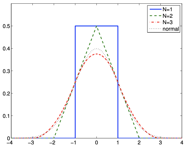
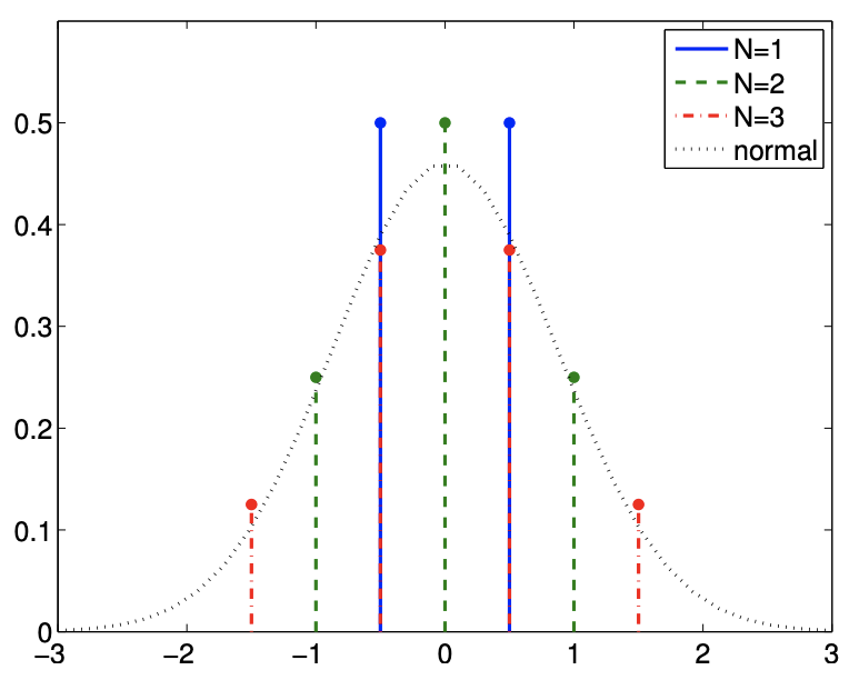
Central Limit Theorem

The ubiquitousness of the normal distribution stems from the central limit theorem. (The normal density is also very convenient, with intuitive location \((\mu)\) and scale \(\left(\sigma^{2}\right)\) parameters.) The central limits theorem states that the sum of a sufficiently larger number of i.i.d. random variables tends to a normal distribution. In other words, if an experiment is repeated a larger number of times, the outcome on average approaches a normal distribution. Specifically, given i.i.d. random variables \(X_{i}, i=1, \ldots, N\), each with the mean \(E\left[X_{i}\right]=\mu\) and variance \(\operatorname{Var}\left[X_{i}\right]=\sigma^{2}\), their sum converges to \[\sum_{i=1}^{N} X_{i} \rightarrow \mathcal{N}\left(\mu N, \sigma^{2} N\right), \quad \text { as } \quad N \rightarrow \infty\]

(a) Sum of uniform random variables

(b) Sum of (shifted) Bernoulli random variables

Figure 9.14: Illustration of the central limit theorem for continuous and discrete random variables.

(There are a number of mathematical hypotheses which must be satisfied.)

To illustrate the theorem, let us consider the sum of uniform random variables \(X_{i} \sim \mathcal{U}(-1 / 2,1 / 2)\). The mean and variance of the random variable are \(E\left[X_{i}\right]=0\) and \(\operatorname{Var}\left[X_{i}\right]=1 / 3\), respectively. By central limit theorem, we expect their sum, \(Z_{N}\), to approach \[Z_{N} \equiv \sum_{i=1}^{N} X_{i} \rightarrow \mathcal{N}\left(\mu N, \sigma^{2} N\right)=\mathcal{N}(0, N / 3) \quad \text { as } \quad N \rightarrow \infty\] The pdf of the sum \(Z_{i}, i=1,2,3\), and the normal distribution \(\left.\mathcal{N}(0, N / 3)\right|_{N=3}=\mathcal{N}(0,1)\) are shown in Figure \(9.14(\mathrm{a})\). Even though the original uniform distribution \((N=1)\) is far from normal and \(N=3\) is not a large number, the pdf for \(N=3\) can be closely approximated by the normal distribution, confirming the central limit theorem in this particular case.

The theorem also applies to discrete random variable. For example, let us consider the sum of (shifted) Bernoulli random variables, \[X_{i}=\left\{\begin{aligned} -1 / 2, & \text { with probability } 1 / 2 \\ 1 / 2, & \text { with probability } 1 / 2 \end{aligned}\right.\] Note that the value that \(X\) takes is shifted by \(-1 / 2\) compared to the standard Bernoulli random variable, such that the variable has zero mean. The variance of the distribution is \(\operatorname{Var}\left[X_{i}\right]=1 / 4\). As this is a discrete distribution, their sum also takes on discrete values; however, Figure \(9.14(\mathrm{~b})\) shows that the probability mass function can be closely approximated by the pdf for the normal distribution.

Generation of Pseudo-Random Numbers

To generate a realization of a random variable \(X\) - also known as a random variate - computationally, we can use a pseudo-random number generator. Pseudo-random number generators are algorithms that generate a sequence of numbers that appear to be random. However, the actual sequence generated is completely determined by a seed - the variable that specifies the initial state of the generator. In other words, given a seed, the sequence of the numbers generated is completely deterministic and reproducible. Thus, to generate a different sequence each time, a pseudo-random number generator is seeded with a quantity that is not fixed; a common choice is to use the current machine time. However, the deterministic nature of the pseudo-random number can be useful, for example, for debugging a code.

A typical computer language comes with a library that produces the standard continuous uniform distribution and the standard normal distribution. To generate other distributions, we can apply the transformations we considered earlier. For example, suppose that we have a pseudorandom number generator that generates the realization of \(U \sim \mathcal{U}(0,1)\), \[u_{1}, u_{2}, \ldots .\] Then, we can generate a realization of a general uniform distribution \(X \sim \mathcal{U}(a, b)\), \[x_{1}, x_{2}, \ldots\] by using the transformation \[x_{i}=a+(b-a) u_{i}, \quad i=1,2, \ldots .\] Similarly, we can generate given a realization of the standard normal distribution \(Z \sim \mathcal{N}(0,1)\), \(z_{1}, z_{2}, \ldots\), we can generate a realization of a general normal distribution \(X \sim \mathcal{N}\left(\mu, \sigma^{2}\right), x_{1}, x_{2}, \ldots\), by \[x_{i}=\mu+\sigma z_{i}, \quad i=1,2, \ldots .\] These two transformations are perhaps the most common.

Finally, if we wish to generate a discrete random number \(Y\) with the probability mass function \[f_{Y}(y)=\left\{\begin{array}{ll} 1 / 2, & y_{1}=0 \\ 1 / 4, & y_{2}=2 \\ 1 / 4, & y_{3}=3 \end{array},\right.\] we can map a realization of the standard continuous uniform distribution \(U \sim \mathcal{U}(0,1), u_{1}, u_{2}, \ldots\), according to \[y_{i}=\left\{\begin{array}{ll} 0, & u_{i} \in[0,1 / 2) \\ 2, & u_{i} \in[1 / 2,3 / 4) \\ 3, & u_{i} \in[3 / 4,1] \end{array} \quad i=1,2, \ldots\right.\] (Many programming languages directly support the uniform pmf.)

More generally, using the procedure described in Example 9.4.6, we can sample a random variable \(Z\) with cumulative distribution function \(F_{Z}\) by mapping realizations of the standard uniform distribution, \(u_{1}, u_{2}, \ldots\) according to \[z_{i}=F_{Z}^{-1}\left(u_{i}\right), \quad i=1,2, \ldots .\] We note that there are other sampling techniques which are even more general (if not always efficient), such as "acceptance-rejection" approaches.