10.4: Cumulative Sample Means

In this subsection, we present a practical means of computing sample means. Let us denote the total number of coin flips by \(n_{\max }\), which defines the size of our sample. We assume \(n_{\exp }=1\), as is almost always the case in practice. We create our sample of size \(n_{\max }\), and then for \(n=1, \ldots, n_{\max }\) we compute a sequence of cumulative sample means. That is, we start with a realization of \(n_{\max }\) coin tosses, \[b_{1}, b_{2}, \ldots, b_{n}, \ldots, b_{n_{\max }}\]

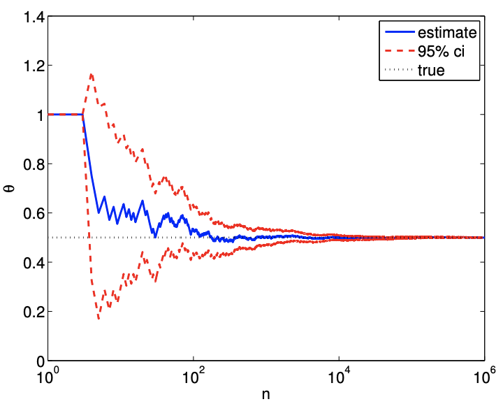
(a) value

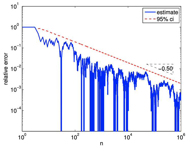
(b) relative error

Figure 10.4: Cumulative sample mean, confidence intervals, and their convergence for a Bernoulli random variable \((\theta=0.5)\).

and then compute the cumulative values,

Note that the random variables \(\bar{B}_{1}, \ldots, \bar{B}_{n_{\max }}\) realized by \(\bar{b}_{1}, \ldots, \bar{b}_{n_{\max }}\) are not independent because the sample means are computed from the same set of realizations; also, the random variable, \([\mathrm{CI}]_{n}\) realized by \([\mathrm{ci}]_{n}\) are not joint with confidence \(\gamma\). However in practice this is a computationally efficient way to estimate the parameter with typically only small loss in rigor. In particular, by plotting \(\hat{\theta}_{n}\) and \([\text { ci }]_{n}\) for \(n=1, \ldots, n_{\max }\), one can deduce the convergence behavior of the simulation. In effect, we only perform one experiment, but we interpret it as \(n_{\max }\) experiments.

Figure \(10.4\) shows an example of computing the sample means and confidence intervals in a cumulative manner. The figure confirms that the estimate converges to the true parameter value of \(\theta=0.5\). The confidence interval is a good indicator of the quality of the solution. The error (and the confidence interval) converges at the rate of \(n^{-1 / 2}\), which agrees with the theory. \[\begin{aligned} & \hat{\theta}_{1}=\bar{b}_{1}=\frac{1}{1} \cdot b_{1} \quad \text { and } \quad[\mathrm{ci}]_{1}=\left[\hat{\theta}_{1}-z_{\gamma} \sqrt{\frac{\hat{\theta}_{1}\left(1-\hat{\theta}_{1}\right)}{1}}, \hat{\theta}_{1}+z_{\gamma} \sqrt{\frac{\hat{\theta}_{1}\left(1-\hat{\theta}_{1}\right)}{1}}\right] \\ & \hat{\theta}_{2}=\bar{b}_{2}=\frac{1}{2}\left(b_{1}+b_{2}\right) \quad \text { and } \quad[\mathrm{ci}]_{2}=\left[\hat{\theta}_{2}-z_{\gamma} \sqrt{\frac{\hat{\theta}_{2}\left(1-\hat{\theta}_{2}\right)}{2}}, \hat{\theta}_{2}+z_{\gamma} \sqrt{\frac{\hat{\theta}_{2}\left(1-\hat{\theta}_{2}\right)}{2}}\right] \\ & \hat{\theta}_{n}=\bar{b}_{n}=\frac{1}{n} \sum_{i=1}^{n} b_{i} \quad \text { and } \quad[\mathrm{ci}]_{n}=\left[\hat{\theta}_{n}-z_{\gamma} \sqrt{\frac{\hat{\theta}_{n}\left(1-\hat{\theta}_{n}\right)}{n}}, \hat{\theta}_{n}+z_{\gamma} \sqrt{\frac{\hat{\theta}_{n}\left(1-\hat{\theta}_{n}\right)}{n}}\right] \\ & \hat{\theta}_{n_{\max }}=\bar{b}_{n_{\max }}=\frac{1}{n} \sum_{i=1}^{n_{\max }} b_{i} \quad \text { and } \quad[\mathrm{ci}]_{n_{\max }}=\left[\hat{\theta}_{n_{\max }}-z_{\gamma} \sqrt{\frac{\hat{\theta}_{n_{\max }}\left(1-\hat{\theta}_{n_{\max }}\right)}{n_{\max }}}, \hat{\theta}_{n_{\max }}+z_{\gamma} \sqrt{\frac{\hat{\theta}_{n_{\max }}\left(1-\hat{\theta}_{n_{\max }}\right)}{n_{\max }}}\right] \text {. } \end{aligned}\]