10.3: Confidence Intervals

Definition

Let us now introduce the concept of confidence interval. The confidence interval is a probabilistic \(a\) posteriori error bound. A posteriori error bounds, as oppose to a priori error bounds, incorporate the information gathered in the experiment in order to assess the error in the prediction.

To understand the behavior of the estimator \(\widehat{\Theta}_{n}\), which is a random variable defined by \[B_{1}, \ldots, B_{n} \quad \Rightarrow \quad \widehat{\Theta}_{n}=\bar{B}_{n}=\frac{1}{n} \sum_{i=1}^{n} B_{i},\] we typically perform (in practice) a single experiment to generate a realization \(\left(b_{1}, \ldots, b_{n}\right)\). Then, we estimate the parameter by a number \(\hat{\theta}_{n}\) given by \[b_{1}, \ldots, b_{n} \quad \Rightarrow \quad \hat{\theta}_{n}=\bar{b}_{n}=\frac{1}{n} \sum_{i=1}^{n} b_{i} .\] A natural question: How good is the estimate \(\hat{\theta}_{n}\) ? How can we quantify the small deviations of \(\widehat{\Theta}_{n}\) from \(\theta\) as \(n\) increases?

To answer these questions, we may construct a confidence interval, [CI], defined by \[[\mathrm{CI}]_{n} \equiv\left[\widehat{\Theta}_{n}-z_{\gamma} \sqrt{\frac{\widehat{\Theta}_{n}\left(1-\widehat{\Theta}_{n}\right)}{n}}, \widehat{\Theta}_{n}+z_{\gamma} \sqrt{\frac{\widehat{\Theta}_{n}\left(1-\widehat{\Theta}_{n}\right)}{n}}\right]\] such that \[P\left(\theta \in[\mathrm{CI}]_{n}\right)=\gamma\left(z_{\gamma}\right) .\] We recall that \(\theta\) is the true parameter; thus, \(\gamma\) is the confidence level that the true parameter falls within the confidence interval. Note that \([\mathrm{CI}]_{n}\) is a random variable because \(\widehat{\Theta}_{n}\) is a random variable.

For a large enough \(n\), a (oft-used) confidence level of \(\gamma=0.95\) results in \(z_{\gamma} \approx 1.96\). In other words, if we use \(z_{\gamma}=1.96\) to construct our confidence interval, there is a \(95 \%\) probability that the true parameter lies within the confidence interval. In general, as \(\gamma\) increases, \(z_{\gamma}\) increases: if we want to ensure that the parameter lies within a confidence interval at a higher level of confidence, then the width of the confidence interval must be increased for a given \(n\). The appearance of \(1 / \sqrt{n}\) in the confidence interval is due to the appearance of the \(1 / \sqrt{n}\) in the standard deviation of the estimator, \(\sigma_{\widehat{\Theta}_{n}}\) : as \(n\) increases, there is less variation in the estimator.

Strictly speaking, the above result is only valid as \(n \rightarrow \infty\) (and \(\theta \notin\{0,1\}\) ), which ensures that \(\widehat{\Theta}_{n}\) approaches the normal distribution by the central limit theorem. Then, under the normality assumption, we can calculate the value of the confidence-level-dependent multiplication factor \(z_{\gamma}\) according to \[z_{\gamma}=\tilde{z}_{(1+\gamma) / 2},\] where \(\tilde{z}_{\alpha}\) is the \(\alpha\) quantile of the standard normal distribution, i.e. \(\Phi\left(\tilde{z}_{\alpha}\right)=\alpha\) where \(\Phi\) is the cumulative distribution function of the standard normal distribution. For instance, as stated above, \(\gamma=0.95\) results in \(z_{0.95}=\tilde{z}_{0.975} \approx 1.96\). A practical rule for determining the validity of the normality assumption is to ensure that \[n \theta>5 \text { and } n(1-\theta)>5 .\] In practice, the parameter \(\theta\) appearing in the rule is replaced by its estimate, \(\hat{\theta}_{n}\); i.e. we check \[n \hat{\theta}_{n}>5 \text { and } n\left(1-\hat{\theta}_{n}\right)>5 .\] In particular, note that for \(\hat{\theta}_{n}=0\) or 1 , we cannot construct our confidence interval. This is not surprising, as, for \(\hat{\theta}_{n}=0\) or 1 , our confidence interval would be of zero length, whereas clearly there is some uncertainty in our prediction. We note that there are binomial confidence intervals that do not require the normality assumption, but they are slightly more complicated and less intuitive. Note also that in addition to the "centered" confidence intervals described here we may also develop one-sided confidence intervals.

Frequentist Interpretation

To get a better insight into the behavior of the confidence interval, let us provide an frequentist interpretation of the interval. Let us perform \(n_{\exp }\) experiments and construct \(n_{\exp }\) realizations of confidence intervals, i.e. \[[\mathrm{ci}]_{n}^{j}=\left[\hat{\theta}_{n}^{j}-z_{\gamma} \sqrt{\frac{\hat{\theta}_{n}^{j}\left(1-\hat{\theta}_{n}^{j}\right)}{n}}, \hat{\theta}_{n}^{j}+z_{\gamma} \sqrt{\frac{\hat{\theta}_{n}^{j}\left(1-\hat{\theta}_{n}^{j}\right)}{n}}\right], \quad j=1, \ldots, n_{\exp },\] where the realization of sample means is given by \[\left(b_{1}, \ldots, b_{n}\right)^{j} \quad \Rightarrow \quad \hat{\theta}^{j}=\frac{1}{n} \sum_{i=1}^{n} b_{i}^{j} .\] Then, as \(n_{\exp } \rightarrow \infty\), the fraction of experiments for which the true parameter \(\theta\) lies inside \([c i]_{n}^{j}\) tends to \(\gamma\).

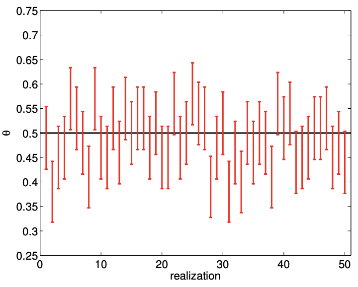
(a) \(80 \%\) confidence

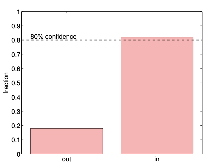
(b) \(80 \%\) confidence in/out

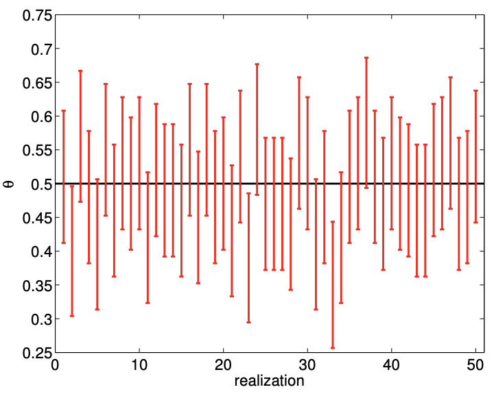
(c) \(95 \%\) confidence

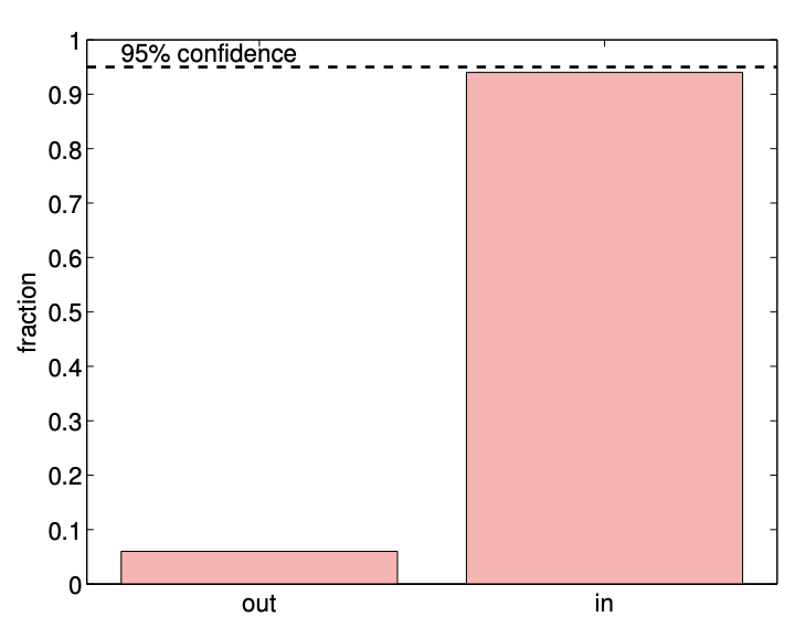
(d) \(95 \%\) confidence in/out

Figure 10.3: An example of confidence intervals for estimating the mean of a Bernoulli random variable \((\theta=0.5)\) using 100 samples.

An example of confidence intervals for estimating the mean of Bernoulli random variable \((\theta=0.5)\) using samples of size \(n=100\) is shown in Figure \(10.3\). In particular, we consider sets of 50 different realizations of our sample (i.e. 50 experiments, each with a sample of size 100) and construct \(80 \%\left(z_{\gamma}=1.28\right)\) and \(95 \%\left(z_{\gamma}=1.96\right)\) confidence intervals for each of the realizations. The histograms shown in Figure 10.3(b) and \(10.3(\mathrm{~d})\) summarize the relative frequency of the true parameter falling in and out of the confidence intervals. We observe that \(80 \%\) and \(95 \%\) confidence intervals include the true parameter \(\theta\) in \(82 \%(9 / 51)\) and \(94 \%(47 / 50)\) of the realizations, respectively; the numbers are in good agreement with the frequentist interpretation of the confidence intervals. Note that, for the same number of samples \(n\), the \(95 \%\) confidence interval has a larger width, as it must ensure that the true parameter lies within the interval with a higher probability.

Convergence

The appearance of \(1 / \sqrt{n}\) convergence of the relative error is due to the \(1 / \sqrt{n}\) dependence in the standard deviation \(\sigma_{\widehat{\Theta}_{n}}\). Thus, the relative error converges in the sense that \[\operatorname{RelErr}_{\theta ; n} \rightarrow 0 \quad \text { as } \quad n \rightarrow \infty .\] However, the convergence rate is slow \[\operatorname{RelErr}_{\theta ; n} \sim n^{-1 / 2},\] i.e. the convergence rate if of order \(1 / 2\) as \(n \rightarrow \infty\). Moreover, note that rare events (i.e. low \(\theta\) ) are difficult to estimate accurately, as \[\operatorname{RelErr}_{\theta ; n} \sim \hat{\theta}_{n}^{-1 / 2} .\] This means that, if the number of experiments is fixed, the relative error in predicting an event that occurs with \(0.1 \%\) probability \((\theta=0.001)\) is 10 times larger than that for an event that occurs with \(10 \%\) probability \((\theta=0.1)\). Combined with the convergence rate of \(n^{-1 / 2}\), it takes 100 times as many experiments to achieve the similar level of relative error if the event is 100 times less likely. Thus, predicting the probability of a rare event is costly.