
10.2: The Sample Mean - An Estimator / Estimate
- Page ID
- 55672

Let us illustrate the idea of sample mean in terms of a coin flip experiment, in which a coin is flipped \(n\) times. Unlike the previous cases, the coin may be unfair, i.e. the probability of heads, \(\theta\), may not be equal to \(1 / 2\). We assume that we do not know the value of \(\theta\), and we wish to estimate \(\theta\) from data collected through \(n\) coin flips. In other words, this is a parameter estimation problem, where the unknown parameter is \(\theta\). Although this chapter serves as a prerequisite for subsequence chapters on Monte Carlo methods - in which we apply probabilistic concepts to calculates areas and more generally integrals - in fact the current chapter focuses on how we might deduce physical parameters from noisy measurements. In short, statistics can be applied either to physical quantities treated as random variables or deterministic quantities which are reinterpreted as random (or pseudo-random).
As in the previous chapter, we associate the outcome of \(n\) flips with a random vector consisting of \(n\) i.i.d. Bernoulli random variables, \[\left(B_{1}, B_{2}, \ldots, B_{n}\right),\] where each \(B_{i}\) takes on the value of 1 with probably of \(\theta\) and 0 with probability of \(1-\theta\). The random variables are i.i.d. because the outcome of one flip is independent of another flip and we are using the same coin.
We define the sample mean of \(n\) coin flips as \[\bar{B}_{n} \equiv \frac{1}{n} \sum_{i=1}^{n} B_{i},\] which is equal to the fraction of flips which are heads. Because \(\bar{B}_{n}\) is a transformation (i.e. sum) of random variables, it is also a random variable. Intuitively, given a large number of flips, we "expect" the fraction of flips which are heads - the frequency of heads - to approach the probability of a head, \(\theta\), for \(n\) sufficiently large. For this reason, the sample mean is our estimator in the context of parameter estimation. Because the estimator estimates the parameter \(\theta\), we will denote it by \(\widehat{\Theta}_{n}\), and it is given by \[\widehat{\Theta}_{n}=\bar{B}_{n}=\frac{1}{n} \sum_{i=1}^{n} B_{i} .\] Note that the sample mean is an example of a statistic - a function of a sample returning a random variable - which, in this case, is intended to estimate the parameter \(\theta\).
We wish to estimate the parameter from a particular realization of coin flips (i.e. a realization of our random sample). For any particular realization, we calculate our estimate as \[\hat{\theta}_{n}=\hat{b}_{n} \equiv \frac{1}{n} \sum_{i=1}^{n} b_{i},\] where \(b_{i}\) is the particular outcome of the \(i\)-th flip. It is important to note that the \(b_{i}, i=1, \ldots, n\), are numbers, each taking the value of either 0 or 1 . Thus, \(\hat{\theta}_{n}\) is a number and not a (random) distribution. Let us summarize the distinctions:
| r.v.? | Description | |
|---|---|---|
| \(\theta\) | no | Parameter to be estimated that governs the behavior of underlying distribution |
| \(\widehat{\Theta}_{n}\) | yes | Estimator for the parameter \(\theta\) |
| \(\hat{\theta}_{n}\) | no | Estimate for the parameter \(\theta\) obtained from a particular realization of our sample |
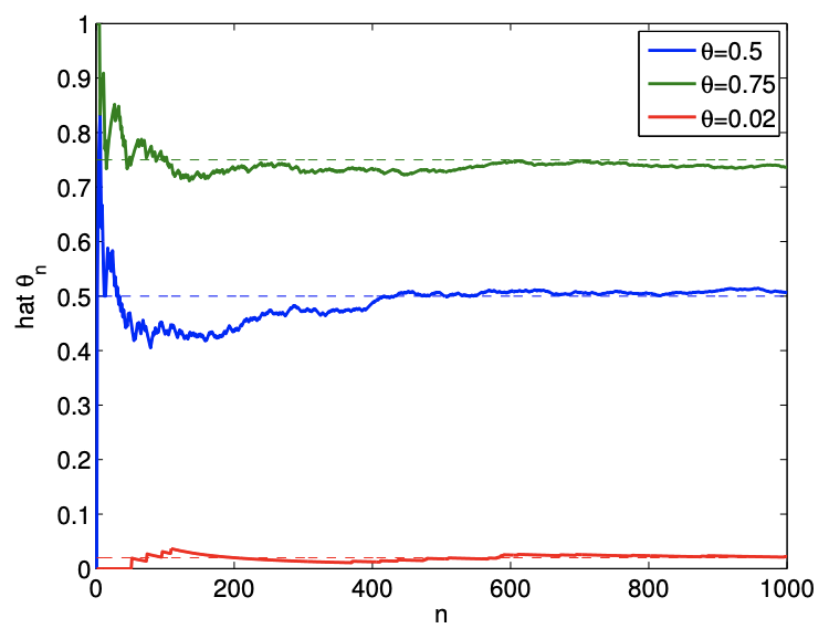
In general, how the random variable \(\widehat{\Theta}_{n}\) is distributed - in particular about \(\theta\) - determines if \(\widehat{\Theta}_{n}\) is a good estimator for the parameter \(\theta\). An example of convergence of \(\hat{\theta}_{n}\) to \(\theta\) with \(n\) is shown in Figure 10.1. As \(n\) increases, \(\hat{\theta}\) converges to \(\theta\) for essentially all realization of \(B_{i}\) ’s. This follows from the fact that \(\widehat{\Theta}_{n}\) is an unbiased estimator of \(\theta\) - an estimator whose expected value is equal to the true parameter. We shall prove this shortly.
To gain a better insight into the behavior of \(\widehat{\Theta}_{n}\), we can construct the empirical distribution of \(\widehat{\Theta}_{n}\) by performing a large number of experiments for a given \(n\). Let us denote the number of
experiments by \(n_{\exp }\). In the first experiment, we work with a realization \(\left(b_{1}, b_{2}, \ldots, b_{n}\right)^{\exp 1}\) and obtain the estimate by computing the mean, i.e. \[\exp 1:\left(b_{1}, b_{2}, \ldots, b_{n}\right)^{\exp 1} \quad \Rightarrow \quad \bar{b}_{n}^{\exp 1}=\frac{1}{n} \sum_{i=1}^{n}\left(b_{i}\right)^{\exp 1} .\] Similarly, for the second experiment, we work with a new realization to obtain \[\exp 2:\left(b_{1}, b_{2}, \ldots, b_{n}\right)^{\exp 2} \quad \Rightarrow \quad \bar{b}_{n}^{\exp 2}=\frac{1}{n} \sum_{i=1}^{n}\left(b_{i}\right)^{\exp 2} .\] Repeating the procedure \(n_{\exp }\) times, we finally obtain \[\exp n_{\exp }:\left(b_{1}, b_{2}, \ldots, b_{n}\right)^{\exp n_{\exp }} \Rightarrow \bar{b}_{n}^{\exp n_{\exp }}=\frac{1}{n} \sum_{i=1}^{n}\left(b_{i}\right)^{\exp n_{\exp }} .\] We note that \(\bar{b}_{n}\) can take any value \(k / n, k=0, \ldots, n\). We can compute the frequency of \(\bar{b}_{n}\) taking on a certain value, i.e. the number of experiments that produces \(\bar{b}_{n}=k / n\).
The numerical result of performing 10,000 experiments for \(n=2,10,100\), and 1000 flips are shown in Figure 10.2. The empirical distribution of \(\widehat{\Theta}_{n}\) shows that \(\widehat{\Theta}_{n}\) more frequently takes on the values close to the underlying parameter \(\theta\) as the number of flips, \(n\), increases. Thus, the numerical experiment confirms that \(\widehat{\Theta}_{n}\) is indeed a good estimator of \(\theta\) if \(n\) is sufficiently large.
Having seen that our estimate converges to the true parameter \(\theta\) in practice, we will now analyze the convergence behavior to the true parameter by relating the sample mean to a binomial distribution. Recall, that the binomial distribution represents the number of heads obtained in flipping a coin \(n\) times, i.e. if \(Z_{n} \sim \mathcal{B}(n, \theta)\), then \[Z_{n}=\sum_{i=1}^{n} B_{i},\] where \(B_{i}, i=1, \ldots, n\), are the i.i.d. Bernoulli random variable representing the outcome of coin flips (each having the probability of head of \(\theta\) ). The binomial distribution and the sample mean are related by \[\widehat{\Theta}_{n}=\frac{1}{n} Z_{n}\]
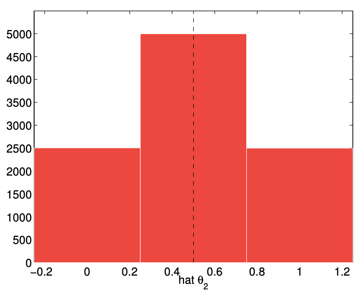
(a) \(n=2\)
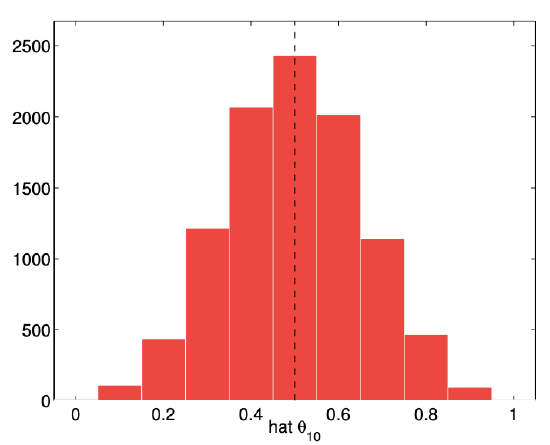
(b) \(n=10\)
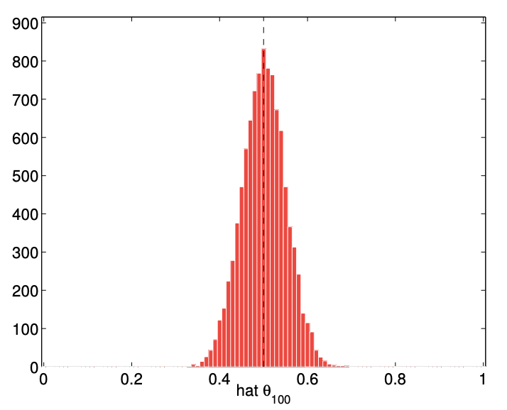
(c) \(n=100\)
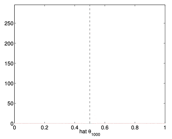
(d) \(n=1000\)
Figure 10.2: Empirical distribution of \(\widehat{\Theta}_{n}\) for \(n=2,10,100\), and 1000 and \(\theta=1 / 2\) obtained from 10,000 experiments.
The mean (a deterministic parameter) of the sample mean (a random variable) is \[E\left[\widehat{\Theta}_{n}\right]=E\left[\frac{1}{n} Z_{n}\right]=\frac{1}{n} E\left[Z_{n}\right]=\frac{1}{n}(n \theta)=\theta .\] In other words, \(\widehat{\Theta}_{n}\) is an unbiased estimator of \(\theta\). The variance of the sample mean is \[\begin{aligned} \operatorname{Var}\left[\widehat{\Theta}_{n}\right] &=E\left[\left(\widehat{\Theta}_{n}-E\left[\widehat{\Theta}_{n}\right]\right)^{2}\right]=E\left[\left(\frac{1}{n} Z_{n}-\frac{1}{n} E\left[Z_{n}\right]\right)^{2}\right]=\frac{1}{n^{2}} E\left[\left(Z_{n}-E\left[Z_{n}\right]\right)^{2}\right] \\ &=\frac{1}{n^{2}} \operatorname{Var}\left[Z_{n}\right]=\frac{1}{n^{2}} n \theta(1-\theta)=\frac{\theta(1-\theta)}{n} . \end{aligned}\] The standard deviation of \(\widehat{\Theta}_{n}\) is \[\sigma_{\hat{\Theta}_{n}}=\sqrt{\operatorname{Var}\left[\widehat{\Theta}_{n}\right]}=\sqrt{\frac{\theta(1-\theta)}{n}} .\] Thus, the standard deviation of \(\widehat{\Theta}_{n}\) decreases with \(n\), and in particular tends to zero as \(1 / \sqrt{n}\). This implies that \(\widehat{\Theta}_{n} \rightarrow \theta\) as \(n \rightarrow \infty\) because it is very unlikely that \(\widehat{\Theta}_{n}\) will take on a value many standard deviations away from the mean. In other words, the estimator converges to the true parameter with the number of flips.