12.1: Calculating an Area

We have seen in Chapter 10 and 11 that parameters that describe probability distributions can be estimated using a finite number of realizations of the random variable and that furthermore we can construct an error bound (in the form of confidence interval) for such an estimate. In this chapter, we introduce Monte Carlo methods to estimate the area (or volume) of implicitly-defined regions. Specifically, we recast the area determination problem as a problem of estimating the mean of a certain Bernoulli distribution and then apply the tools developed in Chapter 10 to estimate the area and also assess errors in our estimate.

Objective

We are given a two-dimensional domain \(D\) in a rectangle \(R=\left[a_{1}, b_{1}\right] \times\left[a_{2}, b_{2}\right]\). We would like to find, or estimate, the area of \(D, A_{D}\). Note that the area of the bounding rectangle, \(A_{R}=\left(b_{1}-a_{1}\right)\left(b_{2}-a_{2}\right)\), is known.

Continuous Uniform Random Variable

Let \(X \equiv\left(X_{1}, X_{2}\right)\) be a uniform random variable over \(R\). We know that, by the definition of uniform distribution, \[f_{X_{1}, X_{2}}\left(x_{1}, x_{2}\right)=\left\{\begin{array}{ll} 1 / A_{R}, & \left(x_{1}, x_{2}\right) \in R \\ 0, & \left(x_{1}, x_{2}\right) \notin R \end{array},\right.\] and we know how to sample from \(f_{X_{1}, X_{2}}\) by using independence and univariate uniform densities. Finally, we can express the probability that \(X\) takes on a value in \(D\) as \[P(X \in D)=\iint_{D} f_{X_{1}, X_{2}}\left(x_{1}, x_{2}\right) d x_{1} d x_{2}=\frac{1}{A_{R}} \iint_{D} d x_{1} d x_{2}=\frac{A_{D}}{A_{R}} .\] Intuitively, this means that the probability of a random "dart" landing in \(D\) is equal to the fraction of the area that \(D\) occupies with respect to \(R\).

Bernoulli Random Variable

Let us introduce a Bernoulli random variable, \[B= \begin{cases}1 & X \in D \text { with probability } \theta \\ 0 & X \notin D \text { with probability } 1-\theta\end{cases}\] But, \[P(X \in D)=A_{D} / A_{R}\] So, by our usual transformation rules, \[\theta \equiv \frac{A_{D}}{A_{R}} .\] In other words, if we can estimate \(\theta\) we can estimate \(A_{D}=A_{R} \theta\). We know how to estimate \(\theta-\) same as coin flips. But, how do we sample \(B\) if we do not know \(\theta\)?

Estimation: Monte Carlo

We draw a sample of random vectors, \[\left(x_{1}, x_{2}\right)_{1},\left(x_{1}, x_{2}\right)_{2}, \ldots,\left(x_{1}, x_{2}\right)_{n}, \ldots,\left(x_{1}, x_{2}\right)_{n_{\max }}\] and then map the sampled pairs to realization of Bernoulli random variables \[\left(x_{1}, x_{2}\right)_{i} \rightarrow b_{i}, \quad i=1, \ldots, n_{\max } .\] Given the realization of Bernoulli random variables, \[b_{1}, \ldots, b_{n}, \ldots, b_{n_{\max }},\] we can apply the technique discussed in Section \(10.4\) to compute the sample means and confidence intervals: for \(n=1, \ldots, n_{\max }\), \[\hat{\theta}_{n}=\bar{b}_{n}=\frac{1}{n} \sum_{i=1}^{n} b_{i} \quad \text { and } \quad[\mathrm{ci}]_{n}=\left[\hat{\theta}_{n}-z_{\gamma} \sqrt{\frac{\hat{\theta}_{n}\left(1-\hat{\theta}_{n}\right)}{n}}, \hat{\theta}_{n}+z_{\gamma} \sqrt{\frac{\hat{\theta}_{n}\left(1-\hat{\theta}_{n}\right)}{n}}\right] .\] Thus, given the mapping from the sampled pairs to Bernoulli variables, we can estimate the parameter.

The only remaining question is how to construct the mapping \(\left(x_{1}, x_{2}\right)_{n} \rightarrow b_{n}, n=1, \ldots, n_{\max }\). The appropriate mapping is, given \(\left(x_{1}, x_{2}\right)_{n} \in R\), \[b_{n}=\left\{\begin{array}{ll} 1, & \left(x_{1}, x_{2}\right)_{n} \in D \\ 0, & \left(x_{1}, x_{2}\right)_{n} \notin D \end{array} .\right.\] To understand why this mapping works, we can look at the random variables: given \(\left(X_{1}, X_{2}\right)_{n}\), \[B_{n}=\left\{\begin{array}{ll} 1, & \left(X_{1}, X_{2}\right)_{n} \in D \\ 0, & \left(X_{1}, X_{2}\right)_{n} \notin D \end{array} .\right.\]

(a) \(n=200\)

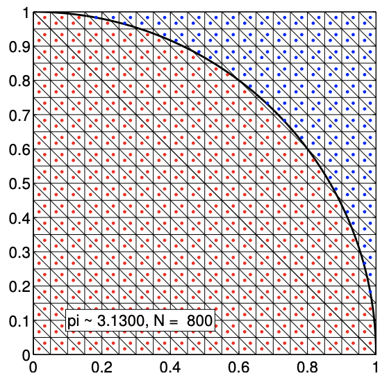
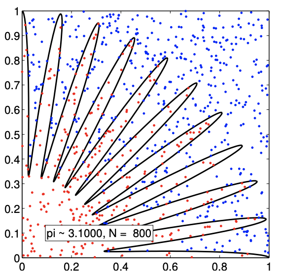
(b) \(n=800\)

Figure 12.1: Estimation of \(\pi\) by Monte Carlo method.

But, \[P\left(\left(X_{1}, X_{2}\right)_{n} \in D\right)=\theta\] SO \[P\left(B_{n}=1\right)=\theta\] for \(\theta=A_{D} / A_{R}\).

This procedure can be intuitively described as

1. Throw \(n\) "random darts" at \(R\)
2. Estimate \(\theta=A_{D} / A_{R}\) by fraction of darts that land in \(D\)

Finally, for \(A_{D}\), we can develop an estimate \[\left(\widehat{A}_{D}\right)_{n}=A_{R} \hat{\theta}_{n}\] and confidence interval \[\left[\mathrm{ci}_{A_{D}}\right]_{n}=A_{R}[\mathrm{ci}]_{n}\]

Example 12.1.1 Estimating \(\pi\)Monte Carlo method

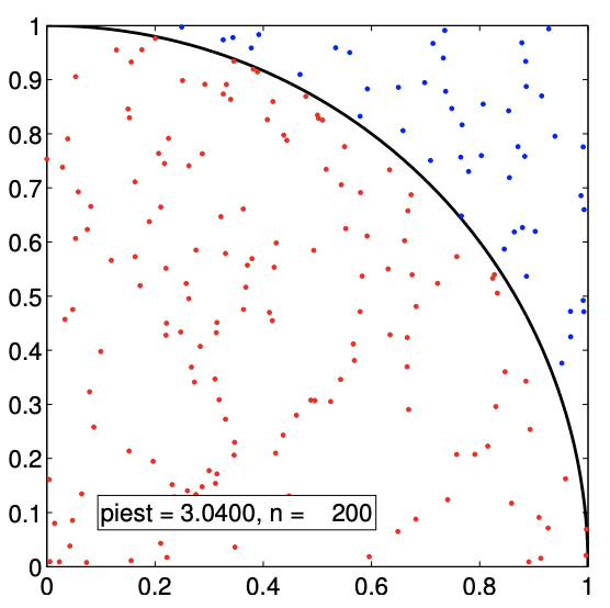
Let us consider an example of estimating the area using Monte Carlo method. In particular, we estimate the area of a circle with unit radius centered at the origin, which has the area of \(\pi r^{2}=\pi\). Noting the symmetry of the problem, let us estimate the area of the quarter circle in the first quadrant and then multiply the area by four to obtain the estimate of \(\pi\). In particular, we sample from the square \[R=[0,1] \times[0,1]\] having the area of \(A_{R}=1\) and aim to determine the area of the quarter circle \(D\) with the area of \(A_{D}\). Clearly, the analytical answer to this problem is \(A_{D}=\pi / 4\). Thus, by estimating \(A_{D}\) using the Monte Carlo method and then multiplying \(A_{D}\) by four, we can estimate the value \(\pi\).

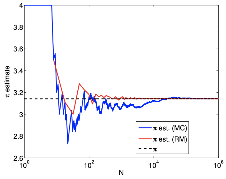
(a) value

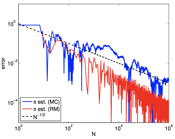
(b) error

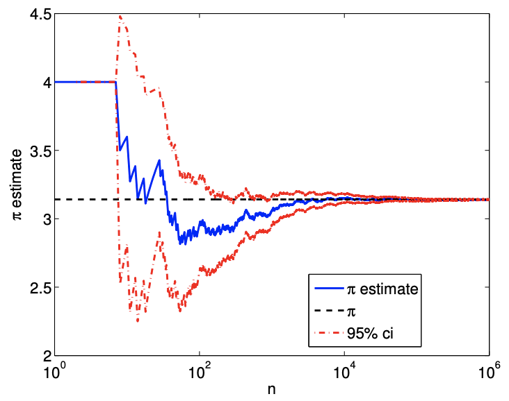
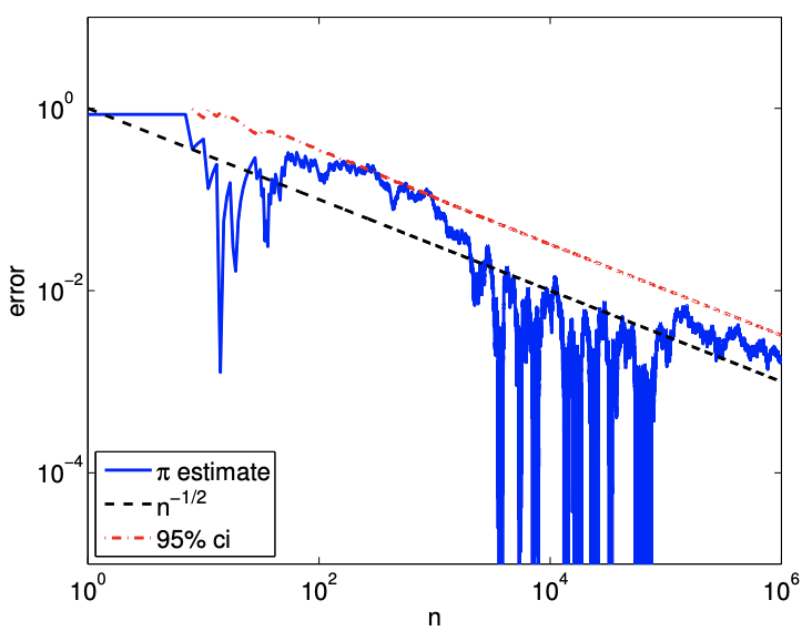
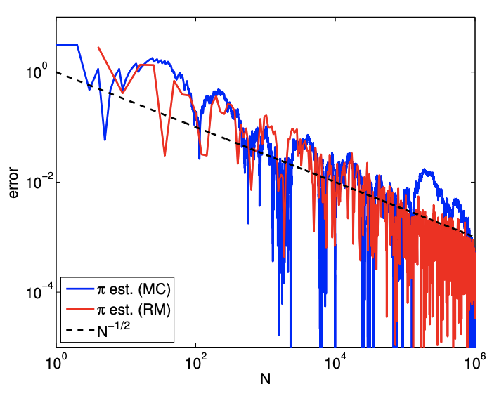
Figure 12.2: Convergence of the \(\pi\) estimate with the number of samples.

The sampling procedure is illustrated in Figure 12.1. To determine whether a given sample \(\left(x_{1}, x_{2}\right)_{n}\) is in the quarter circle, we can compute its distance from the center and determine if the distance is greater than unity, i.e. the Bernoulli variable is assigned according to \[b_{n}=\left\{\begin{array}{ll} 1, & \sqrt{x_{1}^{2}+x_{2}^{2}} \leq 1 \\ 0, & \text { otherwise } \end{array} .\right.\] The samples that evaluates to \(b_{n}=1\) and 0 are plotted in red and blue, respectively. Because the samples are drawn uniformly from the square, the fraction of red dots is equal to the fraction of the area occupied by the quarter circle. We show in Figure \(12.2\) the convergence of the Monte Carlo estimation: we observe the anticipated square-root behavior. Note in the remainder of this section we shall use the more conventional \(N\) rather than \(n\) for sample size.

Estimation: Riemann Sum

As a comparison, let us also use the midpoint rule to find the area of a two-dimensional region \(D\). We first note that the area of \(D\) is equal to the integral of a characteristic function \[\chi\left(x_{1}, x_{2}\right)=\left\{\begin{array}{ll} 1, & \left(x_{1}, x_{2}\right) \in D \\ 0, & \text { otherwise } \end{array},\right.\] over the domain of integration \(R\) that encloses \(D\). For simplicity, we consider rectangular domain \(R=\left[a_{1}, b_{1}\right] \times\left[a_{2}, b_{2}\right]\). We discretize the domain into \(N / 2\) little rectangles, each with the width of \(\left(b_{1}-a_{1}\right) / \sqrt{N / 2}\) and the height of \(\left(b_{2}-a_{2}\right) / \sqrt{N / 2}\). We further divide each rectangle into two right triangles to obtain a triangulation of \(R\). The area of each little triangle \(K\) is \(A_{K}=\) \(\left(b_{1}-a_{1}\right)\left(b_{2}-a_{2}\right) / N\). Application of the midpoint rule to integrate the characteristic function yields \[A_{D} \approx\left(\widehat{A}_{D}^{\mathrm{Rie}}\right)_{N}=\sum_{K} A_{K} \chi\left(x_{c, K}\right)=\sum_{K} \frac{\left(b_{1}-a_{1}\right)\left(b_{2}-a_{2}\right)}{N} \chi\left(x_{c, K}\right),\]

(a) \(N=200\)

(b) \(N=800\)

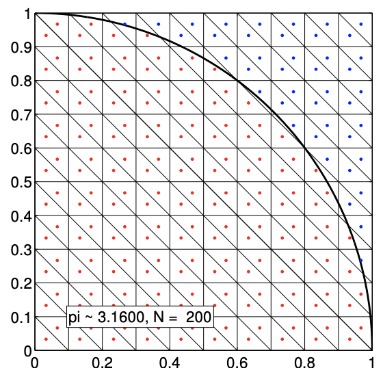
Figure 12.3: Estimation of \(\pi\) by deterministic Riemann sum.

where \(x_{c, K}\) is the centroid (i.e. the midpoint) of the triangle. Noting that \(A_{R}=\left(b_{1}-a_{1}\right)\left(b_{2}-a_{2}\right)\) and rearranging the equation, we obtain \[\left(\widehat{A}_{D}^{\mathrm{Rie}}\right)_{N}=A_{R} \frac{1}{N} \sum_{K} \chi\left(x_{c, K}\right)\] Because the characteristic function takes on either 0 or 1 , the summation is simply equal to the number of times that \(x_{c, K}\) is in the region \(D\). Thus, we obtain our final expression \[\frac{\left(\widehat{A}_{D}^{\mathrm{Rie}}\right)_{N}}{A_{R}}=\frac{\text { number of points in } D}{N}\] Note that the expression is very similar to that of the Monte Carlo integration. The main difference is that the sampling points are structured for the Riemann sum (i.e. the centroid of the triangles).

We can also estimate the error incurred in this process. First, we note that we cannot directly apply the error convergence result for the midpoint rule developed previously because the derivation relied on the smoothness of the integrand. The characteristic function is discontinuous along the boundary of \(D\) and thus is not smooth. To estimate the error, for simplicity, let us assume the domain size is the same in each dimension, i.e. \(a=a_{1}=a_{2}\) and \(b=b_{1}=b_{2}\). Then, the area of each square is \[h^{2}=(b-a)^{2} / N\] Then, \[\left(\widehat{A}_{D}^{\mathrm{Rie}}\right)_{N}=(\text { number of points in } D) \cdot h^{2} .\] There are no errors created by little squares fully inside or fully outside \(D\). All the error is due to the squares that intersect the perimeter. Thus, the error bound can be expressed as \[\begin{aligned} \text { error } & \approx(\text { number of squares that intersect } D) \cdot h^{2} \approx\left(\text { Perimeter }_{D} / h\right) \cdot h^{2} \\ &=\mathcal{O}(h)=\mathcal{O}\left(\sqrt{A_{R} / N}\right) \end{aligned}\]

(a) value

(b) error

Figure 12.4: Convergence of the \(\pi\) estimate with the number of samples using Riemann sum.

Note that this is an example of a priori error estimate. In particular, unlike the error estimate based on the confidence interval of the sample mean for Monte Carlo, this estimate is not constantfree. That is, while we know the asymptotic rate at which the method converges, it does not tell us the actual magnitude of the error, which is problem-dependent. A constant-free estimate typically requires an a posteriori error estimate, which incorporates the information gathered about the particular problem of interest. We show in Figure \(\underline{12.3}\) the Riemann sum grid, and in Figure \(12.4\) the convergence of the Riemann sum approach compared to the convergence of the Monte Carlo approach for our \(\pi\) example.

Example 12.1.2 Integration of a rectangular area

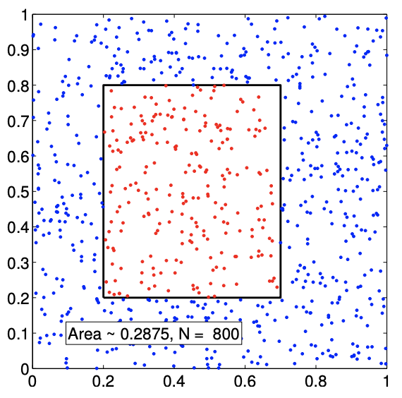
In the case of finding the area of a quarter circle, the Riemann sum performed noticeably better than the Monte Carlo method. However, this is not true in general. To demonstrate this, let us consider integrating the area of a rectangle. In particular, we consider the region \[D=[0.2,0.7] \times[0.2,0.8] .\] The area of the rectangle is \(A_{D}=(0.7-0.2) \cdot(0.8-0.2)=0.3\).

The Monte Carlo integration procedure applied to the rectangular area is illustrated in Figure \(12.5(\mathrm{a})\). The convergence result in Figure \(12.5(\mathrm{~b})\) confirms that both Monte Carlo and Riemann sum converge at the rate of \(N^{-1 / 2}\). Moreover, both methods produce the error of similar level for all ranges of the sample size \(N\) considered.

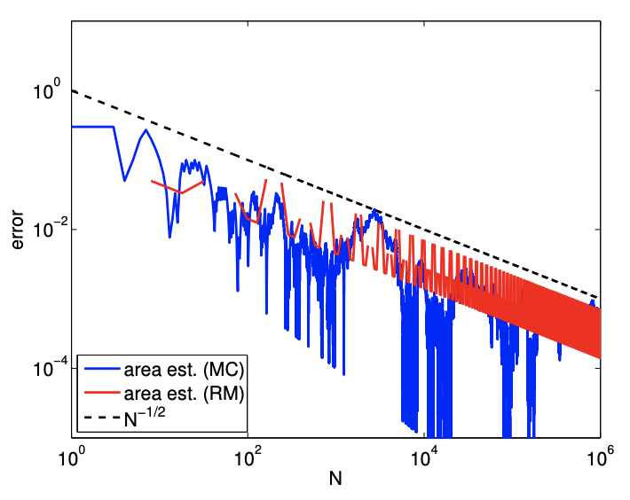
Example 12.1.3 Integration of a complex area

Let us consider estimating the area of a more complex region, shown in Figure 12.6(a). The region \(D\) is implicitly defined in the polar coordinate as \[D=\left\{(r, \theta): r \leq \frac{2}{3}+\frac{1}{3} \cos (4 \beta \theta), 0 \leq \theta \leq \frac{\pi}{2}\right\},\] where \(r=\sqrt{x^{2}+y^{2}}\) and \(\tan (\theta)=y / x\). The particular case shown in the figure is for \(\beta=10\). For any natural number \(\beta\), the area of the region \(D\) is equal to \[A_{D}=\int_{\theta=0}^{\pi / 2} \int_{r=0}^{2 / 3+1 / 3 \cos (4 \beta \theta)} r d r d \theta=\frac{\pi}{8}, \quad \beta=1,2, \ldots .\]

(a) Monte Carlo example

(b) error

Figure 12.5: The geometry and error convergence for the integration over a rectangular area.

(a) Monte Carlo example

(b) error

Figure 12.6: The geometry and error convergence for the integration over a more complex area.

Thus, we can again estimate \(\pi\) by multiplying the estimated area of \(D\) by 8 .

The result of estimating \(\pi\) by approximating the area of \(D\) is shown in Figure \(12.6(b)\). The error convergence plot confirms that both Monte Carlo and Riemann sum converge at the rate of \(N^{-1 / 2}\). In fact, their performances are comparable for this slightly more complex domain.